Session 6: Survival Analysis I
Levi Waldron
session_lecture.RmdLearning objectives and outline
Learning objectives
- Define main types of censoring
- Define the assumption of uninformative censoring
- Define survival function, hazard functions, cumulative event function
- Perform a Kaplan-Meier estimate
- Perform, interpret, and identify assumptions of the logrank test
- Define and calculate potential follow-up time
- Calculate median survival time
Outline
- Introduction to censored data
- Outcome variable: time-to-event
- Types of censored data
- Assumption of uninformative censoring
- Survival function and Kaplan-Meier estimator
- Comparing groups: Log-rank test
- Vittinghoff sections 3.1-3.5
- Tutorial Paper Survival Analysis Part I: Basic concepts and first analyses by Clark, Bradburn, Love, Altman. British Journal of Cancer (2003) 89, 232 – 238
Introduction to censored data
Outcome variable: time to event
- Generally time to the occurrence of a particular event, e.g.
- death
- disease recurrence
- or other experience of interest
- Time: The time from the beginning of an observation period t0
(e.g. surgery) to:
- an event, or
- end of the study, or
- loss of contact or withdrawal from the study
Typical research questions
- What is the median survival time (in years) of patients diagnosed with a certain disease?
- What is the probability of those patients surviving for at least 5 years?
- Are certain personal, behavioral, or clinical characteristics correlated with participant’s chance of survival?
- Is there a survival difference between groups?
- e.g. treatment vs. control
- e.g. exposed vs. unexposed
Special considerations in survival analysis
- Survival data requires special techniques:
- Survival data is generally not normally distributed
- Censoring - observe individuals for differing lengths of time that may or may not result in an “event”
- Censoring is a key challenge in survival analysis. Consider a
clinical study where:
- patient 1 dies 1 month after diagnosis
- patient 2 dies 12 years after diagnosis
- patient 3 is lost to follow-up after 1 month
- patient 4 is still alive after 12 years of follow-up
Question #1: which patients are “censored?”
Question #2: how would you rank these patients in order of disease severity?
Left / right / interval censoring
- right censoring: The event (if it occurs) happens past the end of the observation period
-
left censoring: We observe the presence of a state or
condition but do not know when it began.
- Example: a study investigating the time to recurrence of a cancer following surgical removal of the primary tumor. If the patients were examined 3 months after surgery to determine recurrence, then those who had a recurrence would have a survival time that was left censored because the actual time of recurrence occurred less than 3 months after surgery.
- interval censoring: individuals come in and out of observation.
Classes of uninformative censoring
-
type 1 censoring: The total duration of the study is fixed
- a generalization is fixed censoring: each individual has a potentially different maximum observation time, but still fixed in advance
-
type 2 censoring: The sample is followed as long as
necessary until a pre-specified number of events have occurred
- the length of the study is unknown in advance
- random censoring: the censoring times are independent random variables
These are all analyzed in essentially the same way.
Informative / uninformative censoring
- Uninformative censoring: The most basic assumption we will make is that the censoring of an observation does not provide any information about survival other than that it exceeds the time of the censoring
- Can be violated if, for example, higher risk of death causes study dropout
- Similar to when we assume data missing at random or completely at random
Survival function S(t)
- The Survival function at time t, denoted
,
is the probability of being event-free at t.
- Equivalently, it is the probability that the survival time is greater than t.
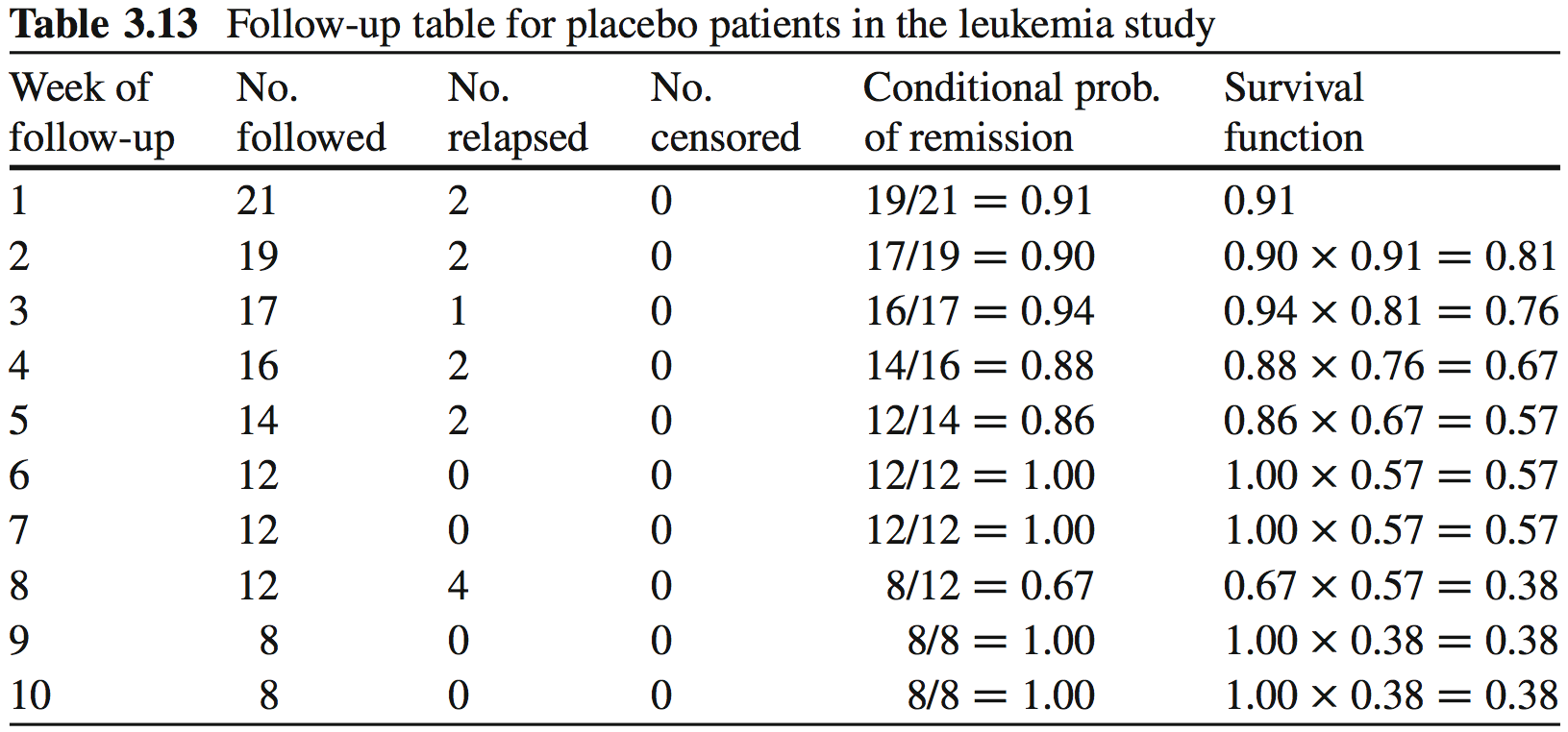
leukemia Example: see leuk.csv
- Study of 6-mercaptopurine (6-MP) maintenance therapy for children in remission from acute lymphoblastic leukemia (ALL)
- 42 patients achieved remission from induction therapy and were then randomized in equal numbers to 6-MP or placebo.
- Survival time studied was from randomization until relapse.
Survival times in weeks for Placebo group:
## [1] 1 1 2 2 3 4 4 5 5 8 8 8 8 11 11 12 12 15 17 22 23Survival times in weeks for Treatment group:
##  [1]  6   6   6   7  10  13  16  22  23   6+  9+ 10+ 11+ 17+ 19+ 20+ 25+ 32+ 32+
## [20] 34+ 35+
Survival function and Kaplan-Meier estimator
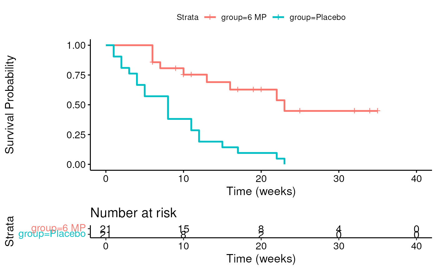
Median Survival Time
Definition: Median Survival Time is the time at which half of a group (sample, population) is expected to experience an event (in this example, death)
- Without censoring, median survival time can be calculated the obvious way
- With censoring, we need to use the Kaplan-Meier estimate of the survival function
## Call: survfit(formula = Surv(time, cens) ~ group, data = leuk)
##
##                n events median 0.95LCL 0.95UCL
## group=6 MP    21      9     23      16      NA
## group=Placebo 21     21      8       4      12
Median Potential Follow-Up Time
Definition: Median Potential Follow-Up Time is the time for which half of a sample would have been expected to be followe, in the absence of events.
- Without any events, median follow-up time can be calculated the obvious way
- With events, a simple median will under-estimate the potential follow-up time. Use a reverse Kaplan-Meier estimate instead:
## Call: survfit(formula = Surv(time, 1 - cens) ~ group, data = leuk)
##
##                n events median 0.95LCL 0.95UCL
## group=6 MP    21     12     25      17      NA
## group=Placebo 21 0 NA NA NANote: Actual median follow-up time is half as long for the placebo group, but there is not reason to believe the potential follow-up times were different
Cumulative Event Function
Definition: The cumulative event function at time t, denoted , is the probability that the event has occurred by time t, or equivalently, the probability that the survival time is less than or equal to t. Note .

Hazard and Cumulative Hazard functions
-
:
hazard function, risk of event at a point in time
- only calculated by software
-
:
cumulative hazard function
- not easily interpretable
- cumulative force of mortality, or the number of events that would be expected for each individual by time t if the event were a repeatable process.
- Will be important next class for Cox Proportional Hazards
Comparing Groups Using the Logrank Test
Log-rank test
-
logrank test is used to compare survival between two or
more groups
- is that the population survival functions are equal at all follow-up times
- is that the population survival functions differ at at least one follow-up time
- logrank test is really just a chi-square test comparing
expected vs. observed number of events in each group.
- Observed is just what we see.
- How to calculate expected?
Log-rank test (cont’d)
Logrank test is just a chisquare test on the observed and expected number of events:
## Call:
## survdiff(formula = Surv(time, cens) ~ group, data = leuk)
##
##                N Observed Expected (O-E)^2/E (O-E)^2/V
## group=6 MP    21        9     19.3      5.46      16.8
## group=Placebo 21       21     10.7      9.77      16.8
##
## Chisq= 16.8 on 1 degrees of freedom, p= 4e-05- Many alternatives are available, but log-rank should be the default
unless you have good reason.
- E.g. Wilcoxon (Breslow), Tarone-Ware, Peto tests
Notes about the Logrank Test
- Non-parametric: no assumptions on the form of
- Log-rank test and K-M curves don’t work with continuous predictors
- Assumes non-informative censoring:
- censoring is unrelated to the likelihood of developing the event of interest
- for each subject, his/her censoring time is statistically independent from their failure time
Summary
- Censoring requires special methods to make full use of the data
- Kaplan-Meier estimate provides non-parametric estimate of the
survival function
- non-parametric meaning that no form of the survival function is assumed; instead it is empirically estimated
- Logrank test provides a non-parametric hypothesis test
- H0: identical survival functions of multiple strata