Session 6 lab exercise: Survival Analysis part 1

Learning objectives

Calculate Kaplan-Meier estimates of survival probability over time
Plot survival curves for censored time-to-event data
Perform and interpret log-rank test
Define “informative” censoring

Exercises

Calculate the follow-up table for 6 MP patients in the leukemia study

library(readr)
leuk <- read_csv("leuk.csv")

## Rows: 42 Columns: 3
## ── Column specification ────────────────────────────────────────────────────────
## Delimiter: ","
## chr (1): group
## dbl (2): time, cens
## 
## ℹ Use `spec()` to retrieve the full column specification for this data.
## ℹ Specify the column types or set `show_col_types = FALSE` to quiet this message.

Plot the Kaplan-Meier estimate of the follow-up table from 1. library(survminer) is recommendable.

library(survival)
library(survminer)

## Loading required package: ggplot2

## Loading required package: ggpubr

## 
## Attaching package: 'survminer'

## The following object is masked from 'package:survival':
## 
##     myeloma

with(leuk, Surv(time, cens))

##  [1]  6   6   6   7  10  13  16  22  23   6+  9+ 10+ 11+ 17+ 19+ 20+ 25+ 32+ 32+
## [20] 34+ 35+  1   1   2   2   3   4   4   5   5   8   8   8   8  11  11  12  12 
## [39] 15  17  22  23

fit <- survminer::surv_fit(Surv(time, cens) ~ group, data = leuk)
survminer::ggsurvplot(fit,
           xlab = "Time (weeks)",
           ylab = "Survival Probability",
           risk.table = TRUE)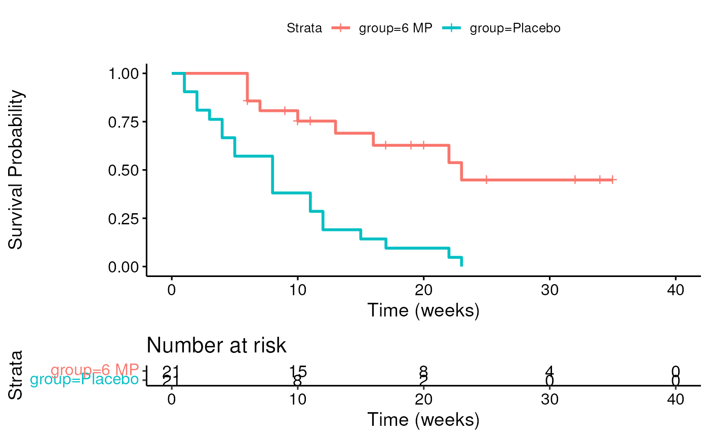

What is the 75th percentile of survival times for the 6 MP group? For the Placebo group? This is the time that 75% of the patients survive. This is also the time at which 25% of patients have had events.

quantile(fit)

## $quantile
##               25 50 75
## group=6 MP    13 23 NA
## group=Placebo  4  8 12
## 
## $lower
##               25 50 75
## group=6 MP     6 16 23
## group=Placebo  2  4  8
## 
## $upper
##               25 50 75
## group=6 MP    NA NA NA
## group=Placebo  8 12 NA

survdiff(Surv(time, cens) ~ group, data = leuk)

## Call:
## survdiff(formula = Surv(time, cens) ~ group, data = leuk)
## 
##                N Observed Expected (O-E)^2/E (O-E)^2/V
## group=6 MP    21        9     19.3      5.46      16.8
## group=Placebo 21       21     10.7      9.77      16.8
## 
##  Chisq= 16.8  on 1 degrees of freedom, p= 4e-05

Suppose you were instructed to cap follow-up times at 20 weeks. Re-do the Kaplan-Meier plot for both groups, and re-do the logrank test.

library(tidyverse)

## ── Attaching core tidyverse packages ──────────────────────── tidyverse 2.0.0 ──
## ✔ dplyr     1.1.3     ✔ stringr   1.5.0
## ✔ forcats   1.0.0     ✔ tibble    3.2.1
## ✔ lubridate 1.9.3     ✔ tidyr     1.3.0
## ✔ purrr     1.0.2     
## ── Conflicts ────────────────────────────────────────── tidyverse_conflicts() ──
## ✖ dplyr::filter() masks stats::filter()
## ✖ dplyr::lag()    masks stats::lag()
## ℹ Use the conflicted package (<http://conflicted.r-lib.org/>) to force all conflicts to become errors

leuknew <- leuk %>% mutate(newtime = pmin(time, 20)) %>% 
  mutate(newcens = ifelse(time <= 20, cens, 0))

Kaplan-Meier plot

fit <- survminer::surv_fit(Surv(newtime, newcens) ~ group, data = leuknew)
survminer::ggsurvplot(fit,
           xlab = "Time (weeks)",
           ylab = "Survival Probability",
           risk.table = TRUE)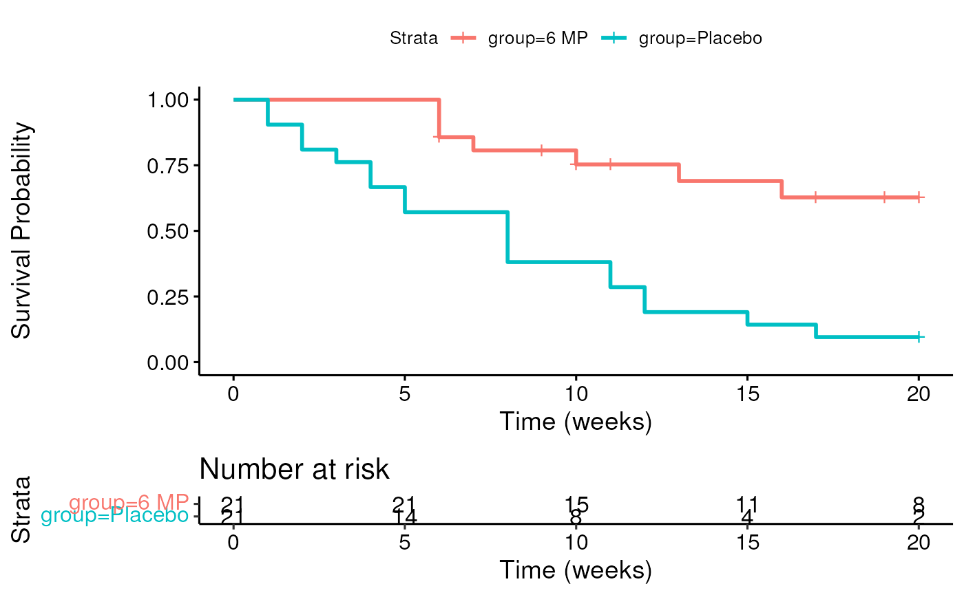

Logrank test

survdiff(Surv(newtime, newcens) ~ group, data = leuknew)

## Call:
## survdiff(formula = Surv(newtime, newcens) ~ group, data = leuknew)
## 
##                N Observed Expected (O-E)^2/E (O-E)^2/V
## group=6 MP    21        7       16      5.05        14
## group=Placebo 21       19       10      8.05        14
## 
##  Chisq= 14  on 1 degrees of freedom, p= 2e-04

Give a hypothetical example of how censoring in this example might be “informative.”

If sicker patients were moved to another hospital where they weren’t followed up on, and were also more likely to relapse, this would be informative censoring.

Levi Waldron