Session 5: loglinear regression part 2

Learning objectives and outline

Learning objectives

Define and identify over-dispersion in count data
Define the negative binomial (NB) distribution and identify applications for it
Define zero-inflated count models
Fit and interpret Poisson and NB, with and without zero inflation

Outline

Review of log-linear Poisson glm
Review of diagnostics and interpretation of coefficients
Over-dispersion
- Negative Binomial distribution
Zero-inflated models

Resources:

Vittinghoff section 8.1-8.3
Short tutorials on regression in R (and Stata, SAS, SPSS, Mplus)
- https://stats.idre.ucla.edu/other/dae/

Review

Components of GLM

Random component specifies the conditional distribution for the response variable - it doesn’t have to be normal but can be any distribution that belongs to the “exponential” family of distributions
Systematic component specifies linear function of predictors (linear predictor)
Link [denoted by g(.)] specifies the relationship between the expected value of the random component and the systematic component, can be linear or nonlinear

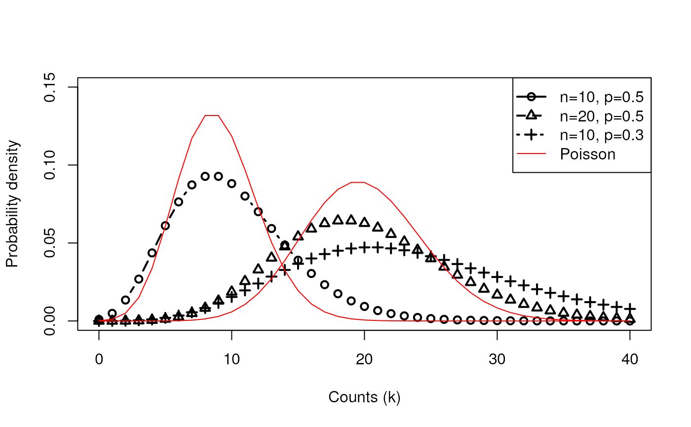
Motivating example: Choice of Distribution

Count data are often modeled as Poisson distributed:
- mean \(\lambda\) is greater than 0
- variance is also \(\lambda\)
- Probability density \(P(k, \lambda) = \frac{\lambda^k}{k!} e^{-\lambda}\)

Poisson model: the GLM

The systematic part of the GLM is: \[ log(\lambda_i) = \beta_0 + \beta_1 \textrm{RACE}_i + \beta_2 \textrm{TRT}_i + \beta_3 \textrm{ALCH}_i + \beta_4 \textrm{DRUG}_i \] Or alternatively: \[ \lambda_i = exp \left( \beta_0 + \beta_1 \textrm{RACE}_i + \beta_2 \textrm{TRT}_i + \beta_3 \textrm{ALCH}_i + \beta_4 \textrm{DRUG}_i \right) \]

The random part is (Recall the \(\lambda_i\) is both the mean and variance of a Poisson distribution): \[ y_i \sim Poisson(\lambda_i) \]

Example: Risky Drug Use Behavior

Outcome is # times the drug user shared a syringe in the past month (shared_syr)
Predictors: sex, ethn, homeless
- filtered to sex “M” or “F”, ethn “White”, “AA”, “Hispanic”

summary(needledat2$shared_syr)

##    Min. 1st Qu.  Median    Mean 3rd Qu.    Max.    NA's 
##   0.000   0.000   0.000   3.122   0.000  60.000       2

var(needledat2$shared_syr, na.rm = TRUE)

## [1] 113.371

Example: Risky Drug Use Behavior

Exploratory plots

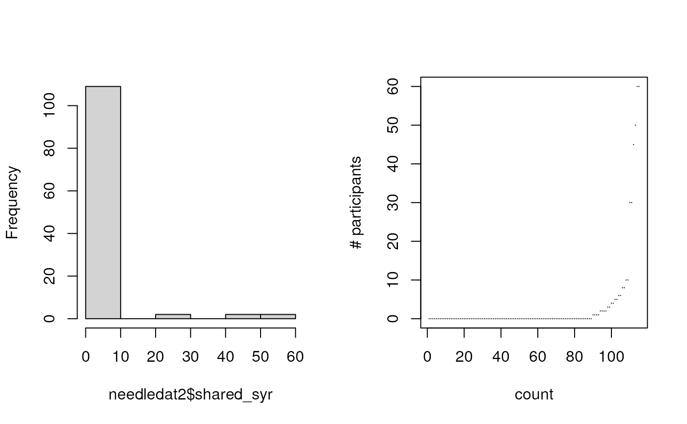
There are a lot of zeros and variance is much greater than mean
- Poisson model is probably not a good fit

Fitting a Poisson model

fit.pois <- glm(shared_syr ~ sex + ethn + homeless,
                data = needledat2,
                family = poisson(link = "log"))

Residuals plots

* Poisson model is definitely not a good fit.

Over-dispersion

When the Poisson model doesn’t fit

Variance > mean (over-dispersion)
- Negative binomial distribution
Excess zeros (zero inflation)
- Can introduce zero-inflation

Negative binomial distribution

The binomial distribution is the number of successes in n trials:
- Roll a die ten times, how many times do you see a 6?
The negative binomial distribution is the number of successes it takes to observe r failures:
- How many times do you have to roll the die to see a 6 ten times?
- Note that the number of rolls is no longer fixed.
- In this example, p=5/6 and a 6 is a “failure”

Negative binomial GLM

One way to parametrize a NB model is with a systematic part equivalent to the Poisson model: \[ log(\lambda_i) = \beta_0 + \beta_1 \textrm{RACE}_i + \beta_2 \textrm{TRT}_i + \beta_3 \textrm{ALCH}_i + \beta_4 \textrm{DRUG}_i \] Or: \[ \lambda_i = exp \left( \beta_0 + \beta_1 \textrm{RACE}_i + \beta_2 \textrm{TRT}_i + \beta_3 \textrm{ALCH}_i + \beta_4 \textrm{DRUG}_i \right) \]

And a random part: \[ y_i \sim NB(\lambda_i, \theta) \]

\(\theta\) is a dispersion parameter that is estimated
When \(\theta = 0\) it is equivalent to Poisson model
MASS::glm.nb() uses this parametrization, dnbinom() does not
The Poisson model can be considered nested within the Negative Binomial model

Negative Binomial Random Distribution

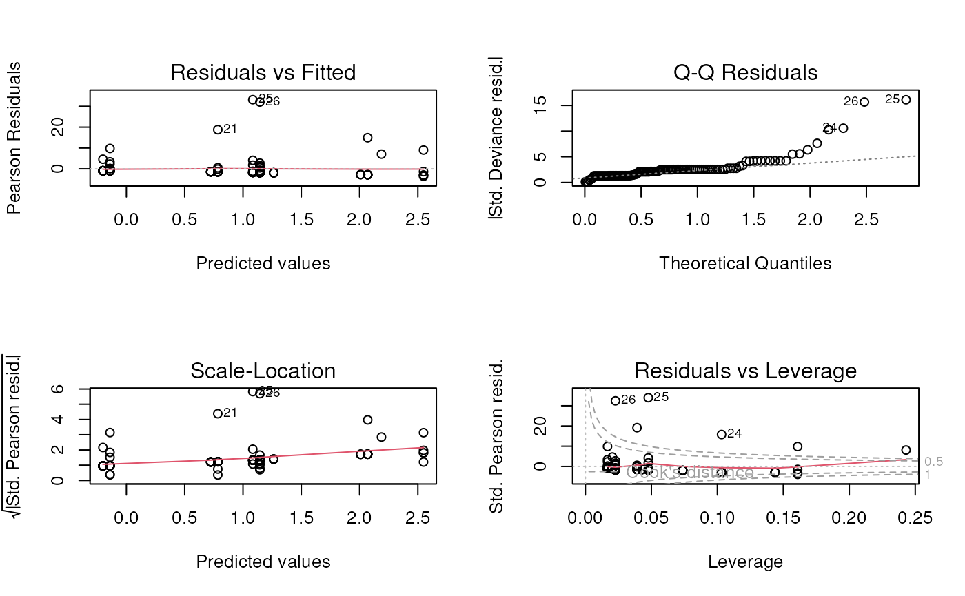
Compare Poisson vs. Negative Binomial

Negative Binomial Distribution has two parameters: # of trials n, and probability of success p

Negative Binomial Regression

library(MASS)
fit.negbin <- MASS::glm.nb(shared_syr ~ sex +
                             ethn + homeless,
                           data = needledat2)

summary(fit.negbin)

## 
## Call:
## MASS::glm.nb(formula = shared_syr ~ sex + ethn + homeless, data = needledat2, 
##     init.theta = 0.07743871374, link = log)
## 
## Coefficients:
##              Estimate Std. Error z value Pr(>|z|)  
## (Intercept)    0.4641     0.8559   0.542   0.5876  
## sexM          -1.0148     0.8294  -1.224   0.2211  
## ethnHispanic   1.3424     1.3201   1.017   0.3092  
## ethnWhite      0.2429     0.7765   0.313   0.7544  
## homelessyes    1.6445     0.7073   2.325   0.0201 *
## ---
## Signif. codes:  0 '***' 0.001 '**' 0.01 '*' 0.05 '.' 0.1 ' ' 1
## 
## (Dispersion parameter for Negative Binomial(0.0774) family taken to be 1)
## 
##     Null deviance: 62.365  on 114  degrees of freedom
## Residual deviance: 56.232  on 110  degrees of freedom
##   (2 observations deleted due to missingness)
## AIC: 306.26
## 
## Number of Fisher Scoring iterations: 1
## 
## 
##               Theta:  0.0774 
##           Std. Err.:  0.0184 
## 
##  2 x log-likelihood:  -294.2550

Likelihood ratio test

Basis: Under \(H_0\): no improvement in fit by more complex model, difference in model residual deviances is \(\chi^2\)-distributed.

Deviance: \(\Delta (\textrm{D}) = -2 * \Delta (\textrm{log likelihood})\)

(ll.negbin <- logLik(fit.negbin))

## 'log Lik.' -147.1277 (df=6)

(ll.pois <- logLik(fit.pois))

## 'log Lik.' -730.0133 (df=5)

pchisq(2 * (ll.negbin - ll.pois), df=1, 
       lower.tail=FALSE)

## 'log Lik.' 1.675949e-255 (df=6)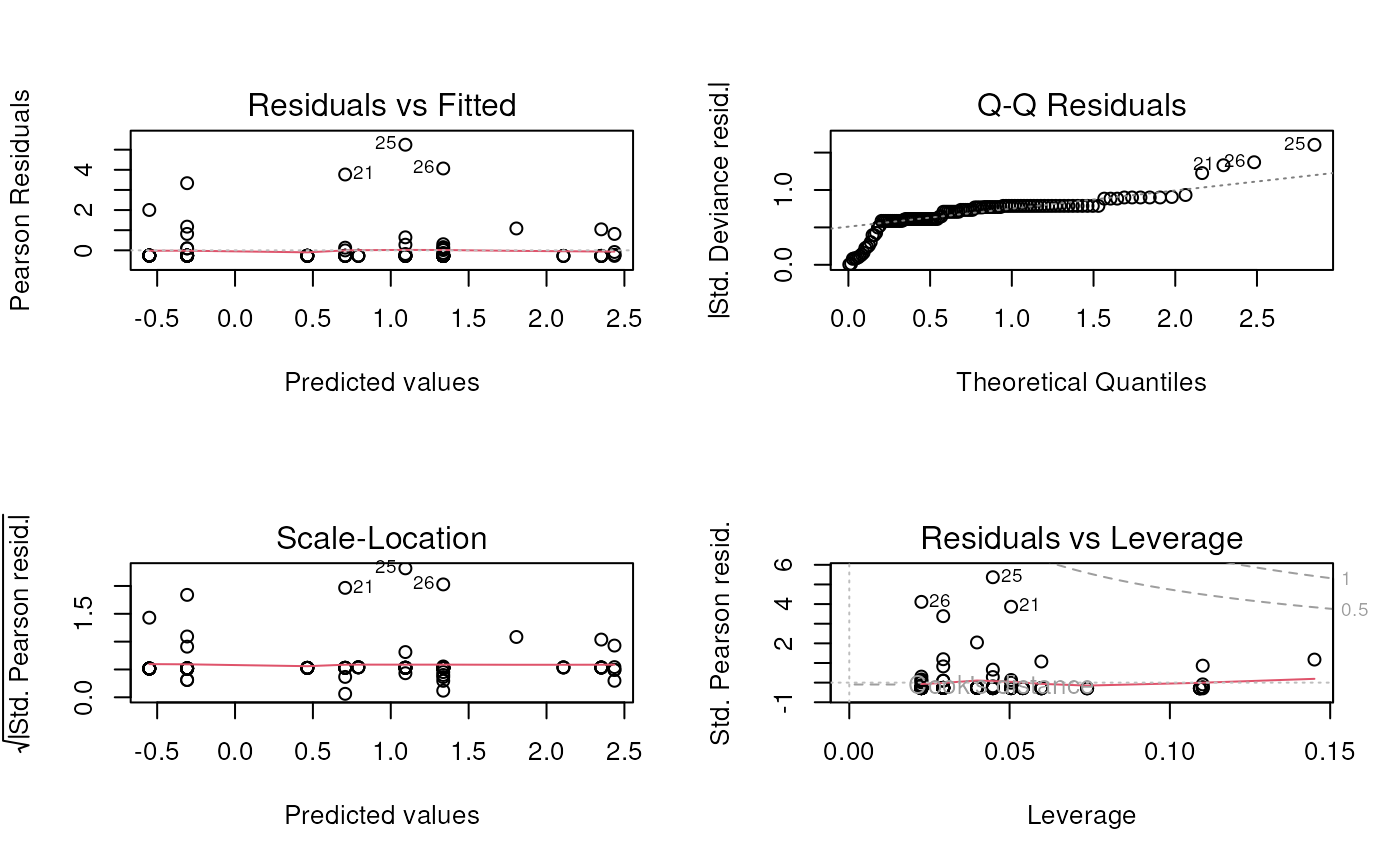

NB regression residuals plots

Zero Inflation

Zero inflated “two-step” models

Step 1: logistic model to determine whether count is zero or Poisson/NB

Step 2: Poisson or NB regression distribution for \(y_i\) not set to zero by 1.

Poisson Distribution with Zero Inflation

Zero-inflated Poisson regression

library(pscl)
fit.ZIpois <-
  pscl::zeroinfl(shared_syr~sex+ethn+homeless,
                 dist = "poisson",
                 data = needledat2)

summary(fit.ZIpois)

## 
## Call:
## pscl::zeroinfl(formula = shared_syr ~ sex + ethn + homeless, data = needledat2, 
##     dist = "poisson")
## 
## Pearson residuals:
##     Min      1Q  Median      3Q     Max 
## -1.0761 -0.5784 -0.4030 -0.3341 10.6835 
## 
## Count model coefficients (poisson with log link):
##              Estimate Std. Error z value Pr(>|z|)    
## (Intercept)    3.2168     0.1796  17.908  < 2e-16 ***
## sexM          -1.4725     0.1442 -10.212  < 2e-16 ***
## ethnHispanic  -0.1524     0.1576  -0.968 0.333244    
## ethnWhite     -0.5236     0.1464  -3.577 0.000348 ***
## homelessyes    1.2034     0.1455   8.268  < 2e-16 ***
## 
## Zero-inflation model coefficients (binomial with logit link):
##              Estimate Std. Error z value Pr(>|z|)   
## (Intercept)   2.06263    0.65227   3.162  0.00157 **
## sexM         -0.05068    0.58252  -0.087  0.93068   
## ethnHispanic -1.76122    0.81177  -2.170  0.03004 * 
## ethnWhite    -0.50187    0.56919  -0.882  0.37792   
## homelessyes  -0.53013    0.48108  -1.102  0.27047   
## ---
## Signif. codes:  0 '***' 0.001 '**' 0.01 '*' 0.05 '.' 0.1 ' ' 1 
## 
## Number of iterations in BFGS optimization: 12 
## Log-likelihood: -299.8 on 10 Df

Zero-inflated Negative Binomial regression

fit.ZInegbin <- 
  pscl::zeroinfl(shared_syr~sex+ethn+homeless,
                         dist = "negbin",
                         data = needledat2)

NOTE: zero-inflation model can include any of your variables as predictors
WARNING Default in zerinfl() function is to use all variables as predictors in logistic model

summary(fit.ZInegbin)

## 
## Call:
## pscl::zeroinfl(formula = shared_syr ~ sex + ethn + homeless, data = needledat2, 
##     dist = "negbin")
## 
## Pearson residuals:
##     Min      1Q  Median      3Q     Max 
## -0.5402 -0.3255 -0.2714 -0.1926  5.1496 
## 
## Count model coefficients (negbin with log link):
##              Estimate Std. Error z value Pr(>|z|)   
## (Intercept)    2.8410     1.1845   2.399  0.01646 * 
## sexM          -2.2282     0.9351  -2.383  0.01718 * 
## ethnHispanic  -0.4123     0.9831  -0.419  0.67492   
## ethnWhite     -0.4299     0.8648  -0.497  0.61908   
## homelessyes    1.9460     0.7103   2.740  0.00615 **
## Log(theta)    -1.1971     0.5159  -2.320  0.02032 * 
## 
## Zero-inflation model coefficients (binomial with logit link):
##              Estimate Std. Error z value Pr(>|z|)  
## (Intercept)    1.6867     0.8465   1.993   0.0463 *
## sexM          -0.9920     0.8016  -1.238   0.2159  
## ethnHispanic -13.1868   281.9134  -0.047   0.9627  
## ethnWhite     -0.7455     0.7304  -1.021   0.3074  
## homelessyes    0.3554     0.7397   0.480   0.6309  
## ---
## Signif. codes:  0 '***' 0.001 '**' 0.01 '*' 0.05 '.' 0.1 ' ' 1 
## 
## Theta = 0.3021 
## Number of iterations in BFGS optimization: 24 
## Log-likelihood: -142.8 on 11 Df

Zero-inflated NB - simplified

Model is much more interpretable if the exposure of interest is not included in the zero-inflation model.
E.g. with HIV status as the only predictor in zero-inflation model:

fit.ZInb2 <- pscl::zeroinfl(shared_syr ~ sex + ethn + 
                        homeless + hiv | hiv,
                      dist = "negbin",
                      data = needledat2)

summary(fit.ZInb2)

## 
## Call:
## pscl::zeroinfl(formula = shared_syr ~ sex + ethn + homeless + hiv | hiv, 
##     data = needledat2, dist = "negbin")
## 
## Pearson residuals:
##     Min      1Q  Median      3Q     Max 
## -0.4299 -0.3646 -0.3559 -0.3299  6.3053 
## 
## Count model coefficients (negbin with log link):
##              Estimate Std. Error z value Pr(>|z|)    
## (Intercept)    3.6685     0.9470   3.874 0.000107 ***
## sexM          -1.7648     0.6205  -2.844 0.004454 ** 
## ethnHispanic  -1.5807     0.7446  -2.123 0.033769 *  
## ethnWhite     -1.1267     0.6924  -1.627 0.103687    
## homelessyes    1.0313     0.5693   1.812 0.070028 .  
## hivpositive   -1.0820     1.0167  -1.064 0.287235    
## hivyes         2.3724     0.7829   3.030 0.002444 ** 
## Log(theta)     0.1395     0.4647   0.300 0.764009    
## 
## Zero-inflation model coefficients (binomial with logit link):
##              Estimate Std. Error z value Pr(>|z|)    
## (Intercept)    1.2163     0.2851   4.265    2e-05 ***
## hivpositive   -0.3493     0.9389  -0.372    0.710    
## hivyes       -17.9654  3065.6271  -0.006    0.995    
## ---
## Signif. codes:  0 '***' 0.001 '**' 0.01 '*' 0.05 '.' 0.1 ' ' 1 
## 
## Theta = 1.1497 
## Number of iterations in BFGS optimization: 12 
## Log-likelihood: -122.5 on 11 Df

Intercept-only ZI model

fit.ZInb3 <-
  pscl::zeroinfl(shared_syr~sex+ethn+homeless|1,
           dist = "negbin",
           data = needledat2)

summary(fit.ZInb3)

## 
## Call:
## pscl::zeroinfl(formula = shared_syr ~ sex + ethn + homeless | 1, data = needledat2, 
##     dist = "negbin")
## 
## Pearson residuals:
##     Min      1Q  Median      3Q     Max 
## -0.3159 -0.3123 -0.3040 -0.2953  5.2940 
## 
## Count model coefficients (negbin with log link):
##              Estimate Std. Error z value Pr(>|z|)  
## (Intercept)   2.08542    1.42671   1.462   0.1438  
## sexM         -1.43809    0.89189  -1.612   0.1069  
## ethnHispanic  0.48130    1.16642   0.413   0.6799  
## ethnWhite    -0.07418    0.81066  -0.092   0.9271  
## homelessyes   1.62076    0.67706   2.394   0.0167 *
## Log(theta)   -1.12538    0.89372  -1.259   0.2080  
## 
## Zero-inflation model coefficients (binomial with logit link):
##             Estimate Std. Error z value Pr(>|z|)
## (Intercept)   0.5211     0.7600   0.686    0.493
## ---
## Signif. codes:  0 '***' 0.001 '**' 0.01 '*' 0.05 '.' 0.1 ' ' 1 
## 
## Theta = 0.3245 
## Number of iterations in BFGS optimization: 13 
## Log-likelihood: -146.8 on 7 Df

Confidence intervals

Use the confint() function for all these models (don’t try to specify which package confint comes from). E.g.:

confint(fit.ZInb3)

##                         2.5 %    97.5 %
## count_(Intercept)  -0.7108906 4.8817285
## count_sexM         -3.1861592 0.3099794
## count_ethnHispanic -1.8048349 2.7674386
## count_ethnWhite    -1.6630517 1.5146931
## count_homelessyes   0.2937565 2.9477701
## zero_(Intercept)   -0.9685313 2.0106906

Residuals vs. fitted values

I invisibly define functions plotpanel1 and plotpanel2 that will work for all types of models (see lab). These use Pearson residuals.

Quantile-quantile plots for residuals

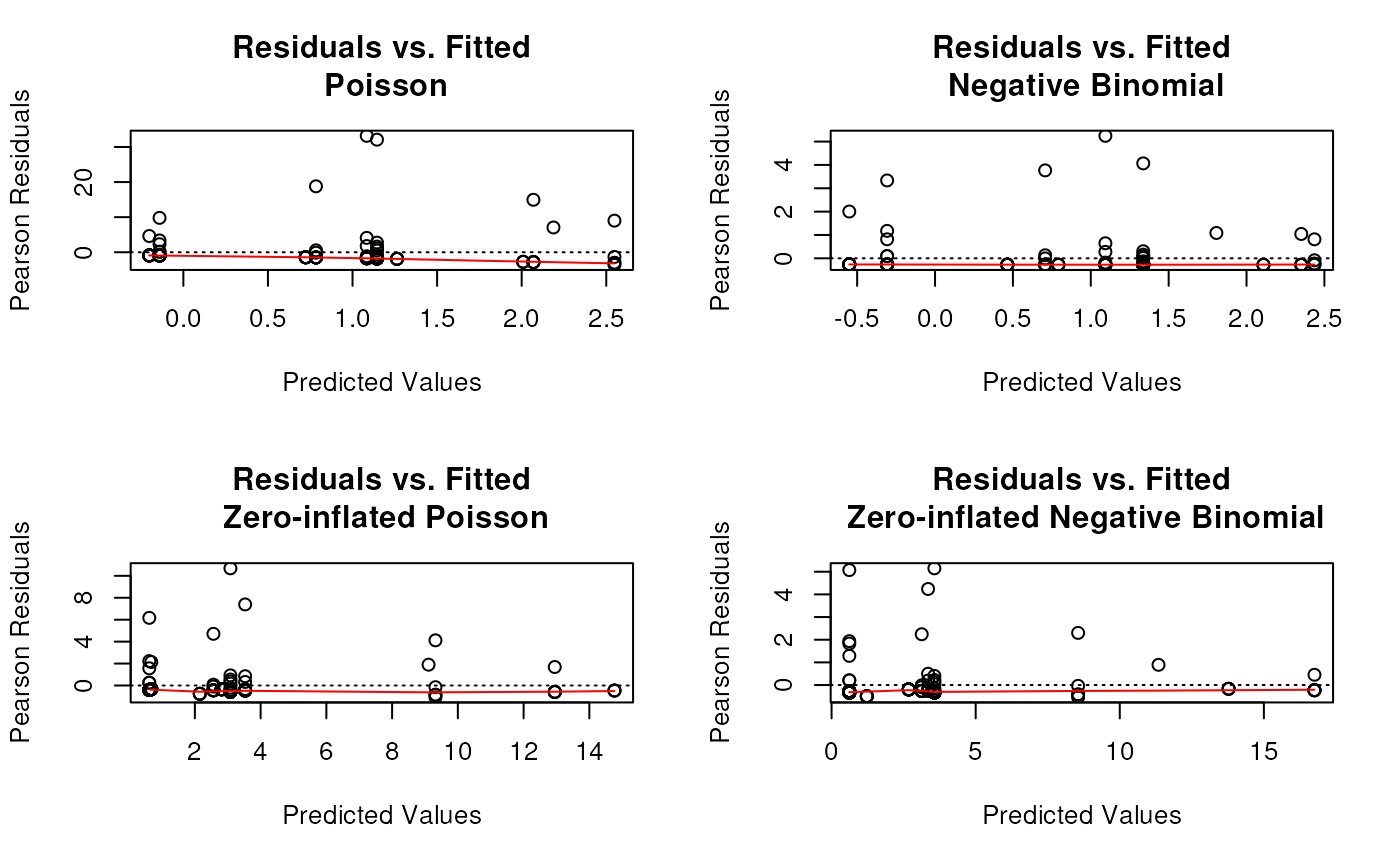
still over-dispersed - ideas?

Summary / Conclusions

These are multiplicative models
Fitting zero-inflated models can be problematic (convergence, over-complicated default models), especially for small samples
Use QQ and residuals plots to assess model fit
Can use LRT to compare nested models

Levi Waldron

Learning objectives and outline

Learning objectives

Outline

Review

Components of GLM

Motivating example: Choice of Distribution

Poisson model: the GLM

Example: Risky Drug Use Behavior

Example: Risky Drug Use Behavior

Fitting a Poisson model

Residuals plots

Over-dispersion

When the Poisson model doesn’t fit

Negative binomial distribution

Negative binomial GLM

Negative Binomial Random Distribution

Compare Poisson vs. Negative Binomial

Negative Binomial Regression

Likelihood ratio test

NB regression residuals plots

Zero Inflation

Zero inflated “two-step” models

Poisson Distribution with Zero Inflation

Zero-inflated Poisson regression

Zero-inflated Negative Binomial regression

Zero-inflated NB - simplified

Intercept-only ZI model

Confidence intervals

Residuals vs. fitted values

Quantile-quantile plots for residuals

Summary / Conclusions