Session 4: loglinear regression part 1

Levi Waldron

Learning objectives and outline

Learning objectives

1. Define log-linear models in GLM framework
2. Identify situations that motivate use of log-linear models
3. Define the Poisson distribution and the log-linear Poisson GLM
4. Identify applications and properties of the Poisson distribution
5. Define multicollinearity and identify resulting issues

Outline

1. Brief review of GLMs
2. Motivating example for log-linear models
3. Poisson log-linear GLM
4. Notes on Multicollinearity

Reading: Vittinghoff textbook chapter 8.1-8.3

Brief review of GLMs

Components of GLM

• Random component specifies the conditional distribution for the response variable - it doesn’t have to be normal but can be any distribution that belongs to the “exponential” family of distributions
• Systematic component specifies linear function of predictors (linear predictor)
• Link [denoted by g(.)] specifies the relationship between the expected value of the random component and the systematic component, can be linear or nonlinear

Linear Regression as GLM

• The model: $y_i = E[y|x] + \epsilon_i = \beta_0 + \beta_1 x_{1i} + \beta_2 x_{2i} + ... + \beta_p x_{pi} + \epsilon_i$

• Random component of $y_i$ is normally distributed: $\epsilon_i \stackrel{iid}{\sim} N(0, \sigma_\epsilon^2)$

• Systematic component (linear predictor): $\beta_0 + \beta_1 x_{1i} + \beta_2 x_{2i} + ... + \beta_p x_{pi}$

• Link function here is the identity link: $g(E(y | x)) = E(y | x)$. We are modeling the mean directly, no transformation.

Logistic Regression as GLM

• The model: $$Logit(P(x)) = log \left( \frac{P(x)}{1-P(x)} \right) = \beta_0 + \beta_1 x_{1i} + \beta_2 x_{2i} + ... + \beta_p x_{pi}$$

• Random component: $y_i$ follows a Binomial distribution (outcome is a binary variable)

• Systematic component: linear predictor $$\beta_0 + \beta_1 x_{1i} + \beta_2 x_{2i} + ... + \beta_p x_{pi}$$

• Link function: logit (Converts Prob -> log-odds) $$g(P(x)) = logit(P(x)) = log\left( \frac{P(x)}{1-P(x)} \right)$$$$P(x) = g^{-1}\left( \beta_0 + \beta_1 x_{1i} + \beta_2 x_{2i} + ... + \beta_p x_{pi} \right)$$

Additive vs. Multiplicative models

• Linear regression is an additive model
  • e.g. for two binary variables $\beta_1 = 1.5$, $\beta_2 = 1.5$.
  • If $x_1=1$ and $x_2=1$, this adds 3.0 to $E(y|x)$
• Logistic regression is a multiplicative model
  • If $x_1=1$ and $x_2=1$, this adds 3.0 to $log(\frac{P}{1-P})$
  • Odds-ratio $\frac{P}{1-P}$ increases 20-fold: $exp(1.5+1.5)$ or $exp(1.5) * exp(1.5)$

Motivating example for log-linear models

Effectiveness of a depression case-management program

• Research question: can a new treatment reduce the number of needed visits to the emergency room, compared to standard care?
• outcome: # of emergency room visits for each patient in the year following initial treatment
• predictors:
  • race (white or nonwhite)
  • treatment (treated or control)
  • amount of alcohol consumption (numerical measure)
  • drug use (numerical measure)

Statistical issues

1. about 1/3 of observations are exactly 0 (did not return to the emergency room within the year)
2. highly nonnormal and cannot be transformed to be approximately normal
3. even $log(y_i + 1)$ transformation will have a “lump” at zero + over 1/2 the transformed data would have values of 0 or $log(2)$
4. a linear regression model would give negative predictions for some covariate combinations
5. some subjects die or cannot be followed up on for a whole year

Poisson log-linear GLM

Towards a reasonable model

• A multiplicative model will allow us to make inference on ratios of mean emergency room usage
• Modeling $log$ of the mean emergency usage ensures positive means, and does not suffer from $log(0)$ problem
• Random component of GLM, or residuals (was $\epsilon_i \stackrel{iid}{\sim} N(0, \sigma_\epsilon^2)$ for linear regression) may still not be normal, but we can choose from other distributions

Proposed model without time

$$log(E[Y_i]) = \beta_0 + \beta_1 \textrm{RACE}_i + \beta_2 \textrm{TRT}_i + \beta_3 \textrm{ALCH}_i + \beta_4 \textrm{DRUG}_i$$ Or equivalently: $$E[Y_i] = exp \left( \beta_0 + \beta_1 \textrm{RACE}_i + \beta_2 \textrm{TRT}_i + \beta_3 \textrm{ALCH}_i + \beta_4 \textrm{DRUG}_i \right)$$ where $E[Y_i]$ is the expected number of emergency room visits for patient i.

• Important note: Modeling $log(E[Y_i])$ is not equivalent to modeling $E(log(Y_i))$

Accounting for follow-up time

Instead, model mean count per unit time: $$\begin{aligned} log(E[Y_i]/t_i) = \beta_0 + \beta_1 \textrm{RACE}_i + \beta_2 \textrm{TRT}_i + \beta_3 \textrm{ALCH}_i + \nonumber \\ \beta_4 \textrm{DRUG}_i \end{aligned}$$

Or equivalently: $$\begin{aligned} log(E[Y_i]) = \beta_0 + \beta_1 \textrm{RACE}_i + \beta_2 \textrm{TRT}_i + \beta_3 \textrm{ALCH}_i + \nonumber \\ \beta_4 \textrm{DRUG}_i + log(t_i) \end{aligned}$$

• $log(t_i)$ is not a covariate, it is called an offset

The Poisson distribution

• Count data are often modeled as Poisson distributed:
  • mean $\lambda$ is greater than 0
  • variance is also $\lambda$
  • Probability density $P(k, \lambda) = \frac{\lambda^k}{k!} e^{-\lambda}$

When the Poisson distribution works

• Individual events are low-probability (small p), but many opportunities (large n)
  • e.g. # 911 calls per day
  • e.g. # emergency room visits
• Approximates the binomial distribution when n is large and p is small
  • e.g. $n > 20$, $np < 5$ or $n(1-p) < 5$
• When mean of residuals is approx. equal to variance

GLM with log-linear link and Poisson error model

• Model the number of counts per unit time as Poisson-distributed + so the expected number of counts per time is $\lambda_i$

$E[Y_i]/t_i = \lambda_i$$log(E[Y_i]/t_i) = log(\lambda_i)$$log(E[Y_i]) = log(\lambda_i) + log(t_i)$

Recalling the log-linear model systematic component: $$\begin{aligned} log(E[Y_i]) = \beta_0 + \beta_1 \textrm{RACE}_i + \beta_2 \textrm{TRT}_i + \beta_3 \textrm{ALCH}_i + \nonumber \\ \beta_4 \textrm{DRUG}_i + log(t_i) \end{aligned}$$

GLM with log-linear link and Poisson error model (cont’d)

Then the systematic part of the GLM is: $$log(\lambda_i) = \beta_0 + \beta_1 \textrm{RACE}_i + \beta_2 \textrm{TRT}_i + \beta_3 \textrm{ALCH}_i + \beta_4 \textrm{DRUG}_i$$ Or alternatively: $$\lambda_i = exp \left( \beta_0 + \beta_1 \textrm{RACE}_i + \beta_2 \textrm{TRT}_i + \beta_3 \textrm{ALCH}_i + \beta_4 \textrm{DRUG}_i \right)$$

Interpretation of coefficients

• Suppose that $\hat \beta_1 = -0.5$ in the fitted model, where $\textrm{RACE}_i=0$ for white and $\textrm{RACE}_i=1$ for non-white.
• The mean rate of emergency room visits per unit time for white relative to non-white, all else held equal, is estimated to be:

$$\frac{exp \left( \beta_0 + 0 + \beta_2 \textrm{TRT}_i + \beta_3 \textrm{ALCH}_i + \beta_4 \textrm{DRUG}_i \right)}{exp \left( \beta_0 - 0.5 + \beta_2 \textrm{TRT}_i + \beta_3 \textrm{ALCH}_i + \beta_4 \textrm{DRUG}_i \right)}$$$$= \frac{e^{\beta_0} e^0 e^{\beta_2 \textrm{TRT}_i} e^{\beta_3 \textrm{ALCH}_i} e^{\beta_4 \textrm{DRUG}_i}} {e^{\beta_0} e^{-0.5} e^{\beta_2 \textrm{TRT}_i} e^{\beta_3 \textrm{ALCH}_i} e^{\beta_4 \textrm{DRUG}_i}}$$$$= \frac{e^0}{e^{-0.5}}$$$$= e^{0.5} \approxeq 1.65$$

Interpretation of coefficients (cont’d)

• If $\hat \beta_1=-0.5$ with whites as the reference group:
  • after adjustment for treatment group, alcohol and drug usage, whites tend to use the emergency room at a rate 1.65 times higher than non-whites.
  • equivalently, the average rate of usage for whites is 65% higher than that for non-whites
• Multiplicative rules apply for other coefficients as well, because they are exponentiated to estimate the mean rate.

Multi-collinearity

What is Multicollinearity?

1. Multicollinearity exists when two or more of the independent variables in regression are moderately or highly correlated.
2. High correlation among continuous predictors or high concordance among categorical predictors
3. Impacts the ability to estimate regression coefficients
   • larger standard errors for regression coefficients
   • ie, coefficients are unstable over repeated sampling
   • exact collinearity produces infinite standard errors on coefficients
4. Can also result in unstable (high variance) prediction models

Identifying multicollinearity

1. Pairwise correlations of data or of model matrix (latter works with categorical variables)
2. Heat maps
3. Variance Inflation Factor (VIF) of regression coefficients

Example: US Judge Ratings dataset

See ?USJudgeRatings for dataset, ?pairs for plot code:

## Warning in par(usr): argument 1 does not name a graphical parameter
## Warning in par(usr): argument 1 does not name a graphical parameter
## Warning in par(usr): argument 1 does not name a graphical parameter
## Warning in par(usr): argument 1 does not name a graphical parameter
## Warning in par(usr): argument 1 does not name a graphical parameter
## Warning in par(usr): argument 1 does not name a graphical parameter
## Warning in par(usr): argument 1 does not name a graphical parameter
## Warning in par(usr): argument 1 does not name a graphical parameter
## Warning in par(usr): argument 1 does not name a graphical parameter
## Warning in par(usr): argument 1 does not name a graphical parameter
## Warning in par(usr): argument 1 does not name a graphical parameter
## Warning in par(usr): argument 1 does not name a graphical parameter
## Warning in par(usr): argument 1 does not name a graphical parameter
## Warning in par(usr): argument 1 does not name a graphical parameter
## Warning in par(usr): argument 1 does not name a graphical parameter
## Warning in par(usr): argument 1 does not name a graphical parameter
## Warning in par(usr): argument 1 does not name a graphical parameter
## Warning in par(usr): argument 1 does not name a graphical parameter
## Warning in par(usr): argument 1 does not name a graphical parameter
## Warning in par(usr): argument 1 does not name a graphical parameter
## Warning in par(usr): argument 1 does not name a graphical parameter
## Warning in par(usr): argument 1 does not name a graphical parameter
## Warning in par(usr): argument 1 does not name a graphical parameter
## Warning in par(usr): argument 1 does not name a graphical parameter
## Warning in par(usr): argument 1 does not name a graphical parameter
## Warning in par(usr): argument 1 does not name a graphical parameter
## Warning in par(usr): argument 1 does not name a graphical parameter
## Warning in par(usr): argument 1 does not name a graphical parameter
## Warning in par(usr): argument 1 does not name a graphical parameter
## Warning in par(usr): argument 1 does not name a graphical parameter
## Warning in par(usr): argument 1 does not name a graphical parameter
## Warning in par(usr): argument 1 does not name a graphical parameter
## Warning in par(usr): argument 1 does not name a graphical parameter
## Warning in par(usr): argument 1 does not name a graphical parameter
## Warning in par(usr): argument 1 does not name a graphical parameter
## Warning in par(usr): argument 1 does not name a graphical parameter
## Warning in par(usr): argument 1 does not name a graphical parameter
## Warning in par(usr): argument 1 does not name a graphical parameter
## Warning in par(usr): argument 1 does not name a graphical parameter
## Warning in par(usr): argument 1 does not name a graphical parameter
## Warning in par(usr): argument 1 does not name a graphical parameter
## Warning in par(usr): argument 1 does not name a graphical parameter
## Warning in par(usr): argument 1 does not name a graphical parameter
## Warning in par(usr): argument 1 does not name a graphical parameter
## Warning in par(usr): argument 1 does not name a graphical parameter
## Warning in par(usr): argument 1 does not name a graphical parameter
## Warning in par(usr): argument 1 does not name a graphical parameter
## Warning in par(usr): argument 1 does not name a graphical parameter
## Warning in par(usr): argument 1 does not name a graphical parameter
## Warning in par(usr): argument 1 does not name a graphical parameter
## Warning in par(usr): argument 1 does not name a graphical parameter
## Warning in par(usr): argument 1 does not name a graphical parameter
## Warning in par(usr): argument 1 does not name a graphical parameter
## Warning in par(usr): argument 1 does not name a graphical parameter
## Warning in par(usr): argument 1 does not name a graphical parameter
## Warning in par(usr): argument 1 does not name a graphical parameter
## Warning in par(usr): argument 1 does not name a graphical parameter
## Warning in par(usr): argument 1 does not name a graphical parameter
## Warning in par(usr): argument 1 does not name a graphical parameter
## Warning in par(usr): argument 1 does not name a graphical parameter
## Warning in par(usr): argument 1 does not name a graphical parameter
## Warning in par(usr): argument 1 does not name a graphical parameter
## Warning in par(usr): argument 1 does not name a graphical parameter
## Warning in par(usr): argument 1 does not name a graphical parameter
## Warning in par(usr): argument 1 does not name a graphical parameter
## Warning in par(usr): argument 1 does not name a graphical parameter

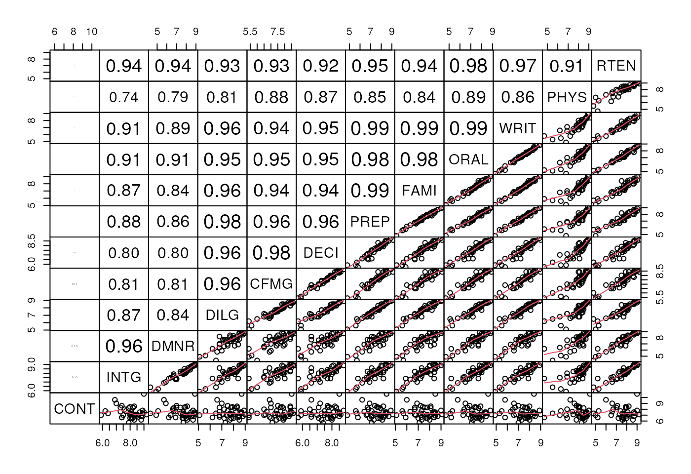
**Pairwise scatterplot of continuous variables in US Judge Ratings dataset

Example: iris dataset

One categorical variable, so use model matrix. Make a simple heatmap.

mm <- model.matrix( ~ ., data = iris)
pheatmap::pheatmap(cor(mm[, -1]), #-1 gets rid of intercept column
  color = colorRampPalette(c("#f0f0f0", "#bdbdbd", "#636363"))(100))

Note: multicollinearity exists between multiple predictors, not between predictor and outcome

Example: iris dataset

Confirm what in iris dataset using Variance Inflation Factor of a linear regression model:

fit <- lm(Sepal.Width ~ ., data = iris)
car::vif(fit)

##                   GVIF Df GVIF^(1/(2*Df))
## Sepal.Length  6.124653  1        2.474804
## Petal.Length 45.132550  1        6.718076
## Petal.Width  18.373804  1        4.286468
## Species      32.701564  2        2.391344

Approaches for dealing with multicollinearity

Options:

1. Select a representative variable
2. Average variables
3. Principal Component Analysis or other dimension reducuction
4. For prediction modeling, special methods like penalized regression, Support Vector Machines, …

Conclusions

Conclusions

1. Log-linear models are appropriate for non-negative, skewed count data
   • probability of each event is low
2. The coefficients of log-linear models are multiplicative
3. An offset term can account for varying follow-up time or otherwise varying opportunity to be counted
4. Poisson distribution is limit of binomial distribution with high number of trials, low probability
5. Inference from log-linear models is sensitive to the choice of error model (assumption on the distribution of residuals)
6. We will cover other options next week for when the Poisson error model doesn’t fit:
   • Variance proportional to mean, instead of equal
   • Negative Binomial
   • Zero Inflation