Session 4 lab exercise: Poisson log-linear regression

Learning objectives

Simulate Poisson-distributed data with a relevant covariate
Fit a Poisson log-linear GLM
Create and interpret diagnostic plots for a log-linear GLM
Use analysis of deviance to compare two log-linear GLMs
Practice recoding and creating tables and plots

Exercises

Simulate count data from a Poisson distribution (for example number of hospital visits by persons over 70 in a 3-year period), where:
1. 10,000 persons annotated with “race” as “white” or “non-white”
2. “white” persons have an average of 3.5 hospital visits during this time period
3. “non-white” persons have an average of 3 hospital visits

library(tidyverse)

## ── Attaching core tidyverse packages ──────────────────────── tidyverse 2.0.0 ──
## ✔ dplyr     1.1.3     ✔ readr     2.1.4
## ✔ forcats   1.0.0     ✔ stringr   1.5.0
## ✔ ggplot2   3.4.4     ✔ tibble    3.2.1
## ✔ lubridate 1.9.3     ✔ tidyr     1.3.0
## ✔ purrr     1.0.2     
## ── Conflicts ────────────────────────────────────────── tidyverse_conflicts() ──
## ✖ dplyr::filter() masks stats::filter()
## ✖ dplyr::lag()    masks stats::lag()
## ℹ Use the conflicted package (<http://conflicted.r-lib.org/>) to force all conflicts to become errors

set.seed(1)
N <- 10000
simdat <- data.frame(race = sample(c("white", "non-white"), N, replace = TRUE)) %>%
  mutate(race = factor(race, levels = c("white", "non-white"))) %>%
  mutate(y = rpois(N, lambda = ifelse(race == "white", 3.5, 3.0)))

Fit a log-linear Poisson model of count outcomes with “race” as the predictor. Note, in this context I tend to use the terms “predictor” and “covariate” interchangeably, to mean any variable used as a predictor in the regression model.

fit <- glm(y ~ race, data = simdat, family = poisson(link = "log"))
summary(fit)

## 
## Call:
## glm(formula = y ~ race, family = poisson(link = "log"), data = simdat)
## 
## Coefficients:
##                Estimate Std. Error z value Pr(>|z|)    
## (Intercept)    1.254710   0.007564  165.88   <2e-16 ***
## racenon-white -0.161428   0.011137  -14.49   <2e-16 ***
## ---
## Signif. codes:  0 '***' 0.001 '**' 0.01 '*' 0.05 '.' 0.1 ' ' 1
## 
## (Dispersion parameter for poisson family taken to be 1)
## 
##     Null deviance: 11041  on 9999  degrees of freedom
## Residual deviance: 10831  on 9998  degrees of freedom
## AIC: 39419
## 
## Number of Fisher Scoring iterations: 5

Use a chi-square test on deviance residuals to test null hypothesis of no relationship between mean hospital visits and race.

The difference in total deviance between two nested models is \(\chi^2\) distributed under \(H_0\) that the more complex model is no better at explaining the response.
- The difference in deviance residuals is (11041 - 10831) = 210, with a difference of 1 degrees of freedom.

The critical threshold for rejection at p=0.05 is:

qchisq(0.95, df=1)

## [1] 3.841459

So we reject \(H_0\)

BEWARE OF MISSING DATA: THIS IS SAFER

fit0 <- glm(y ~ 1, data = simdat, family = poisson(link = "log"))
anova(fit0, fit, test = "LRT")

## Analysis of Deviance Table
## 
## Model 1: y ~ 1
## Model 2: y ~ race
##   Resid. Df Resid. Dev Df Deviance  Pr(>Chi)    
## 1      9999      11042                          
## 2      9998      10831  1   210.76 < 2.2e-16 ***
## ---
## Signif. codes:  0 '***' 0.001 '**' 0.01 '*' 0.05 '.' 0.1 ' ' 1

Create and discuss standard fit diagnostics plots

Example: Risky Drug Use Behavior

Download the “needle_sharing” dataset (see Vittinghoff 8.3.1)
Outcome is # times the drug user shared a syringe in the past month (shared_syr)
Predictors: sex, ethn, homeless

library(readxl)
needledat <- read_excel("needle_sharing.xlsx")
summary(needledat$shared_syr)

##    Min. 1st Qu.  Median    Mean 3rd Qu.    Max.    NA's 
##   0.000   0.000   0.000   2.976   0.000  60.000       5

var(needledat$shared_syr, na.rm=TRUE)

## [1] 106.5978

Some recoding:

suppressPackageStartupMessages(library(dplyr))
needledat_cleaned <-
  mutate(needledat,
    homeless = factor(homeless, levels = 0:1, labels = c("No", "Yes")),
    sex = factor(sex, levels = c("M", "F"), labels = c("Male", "Female")),
    ethnicity = factor(ethn)
  ) %>%
  select(all_of(c("shared_syr", "ethnicity", "sex", "homeless")))

Create a table of the risky drug use behavior dataset

library(table1)

## 
## Attaching package: 'table1'

## The following objects are masked from 'package:base':
## 
##     units, units<-

table1(~ ., data = needledat_cleaned)

	Overall (N=128)
shared_syr
Mean (SD)	2.98 (10.3)
Median [Min, Max]	0 [0, 60.0]
Missing	5 (3.9%)
ethnicity
AA	36 (28.1%)
Asian	1 (0.8%)
Filipino	2 (1.6%)
Hispanic	10 (7.8%)
Indian	1 (0.8%)
Indian & White	1 (0.8%)
White	76 (59.4%)
White & Hispa	1 (0.8%)
sex
Male	97 (75.8%)
Female	30 (23.4%)
Missing	1 (0.8%)
homeless
No	63 (49.2%)
Yes	61 (47.7%)
Missing	4 (3.1%)

Plots of Risky Drug Use Behavior

Create a histogram number of syringe uses
Create a scatter plot of number of syringe uses versus rank of number of syringe uses

library(ggplot2)
ggplot(needledat, aes(shared_syr)) +
  geom_histogram() +
  labs(title = "Counts of Syringe Sharing Incidents Per Person") +
  xlab("Number of Incidents") +
  ylab("Number of people with that count")

## `stat_bin()` using `bins = 30`. Pick better value with `binwidth`.

## Warning: Removed 5 rows containing non-finite values (`stat_bin()`).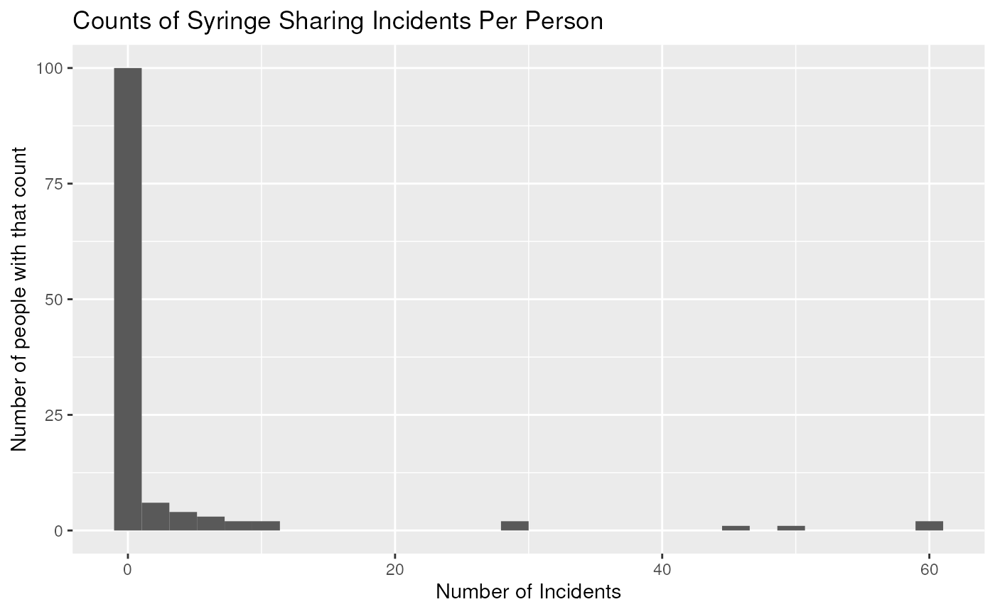

library(dplyr)
mutate(needledat, rnk = rank(shared_syr, ties.method = "first")) %>%
  ggplot(aes(x = rnk, y = shared_syr)) +
  geom_point() +
  labs(title = "Count vs Rank Count of Syringe Sharing Incidents") +
  xlab("rank of count") +
  ylab("count of syringe sharing")

## Warning: Removed 5 rows containing missing values (`geom_point()`).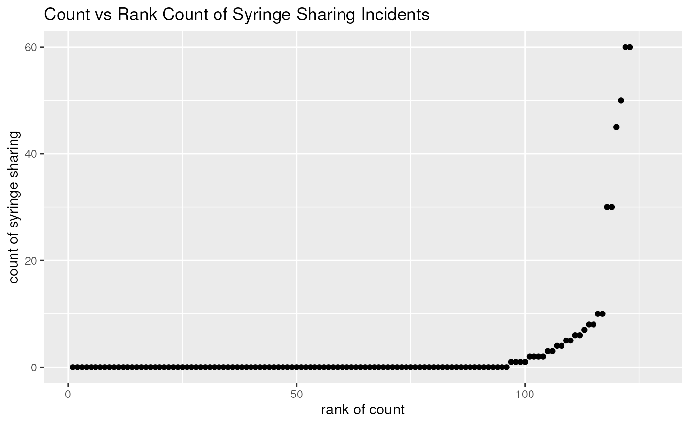

There are a lot of zeros - Poisson model is not a good fit

Fit a Poisson model to the risky drug use behavior dataset anyways

Even though we know it is a bad fit

fit.pois <- glm(shared_syr ~ sex + ethn + homeless,
                data = needledat,
                family = poisson(link = "log"))
summary(fit.pois)

## 
## Call:
## glm(formula = shared_syr ~ sex + ethn + homeless, family = poisson(link = "log"), 
##     data = needledat)
## 
## Coefficients:
##                     Estimate Std. Error z value Pr(>|z|)    
## (Intercept)          0.72332    0.14462   5.002 5.69e-07 ***
## sexM                -0.92480    0.12133  -7.622 2.50e-14 ***
## sexTrans           -15.08655  773.78384  -0.019   0.9844    
## ethnFilipino       -14.52887  510.68253  -0.028   0.9773    
## ethnHispanic         1.46454    0.16004   9.151  < 2e-16 ***
## ethnIndian         -14.10111  773.78385  -0.018   0.9855    
## ethnIndian & White -15.02591  773.78384  -0.019   0.9845    
## ethnWhite            0.06064    0.13348   0.454   0.6496    
## ethnWhite & Hispa    0.86195    0.39872   2.162   0.0306 *  
## homeless             1.28543    0.12664  10.150  < 2e-16 ***
## ---
## Signif. codes:  0 '***' 0.001 '**' 0.01 '*' 0.05 '.' 0.1 ' ' 1
## 
## (Dispersion parameter for poisson family taken to be 1)
## 
##     Null deviance: 1621.9  on 120  degrees of freedom
## Residual deviance: 1364.8  on 111  degrees of freedom
##   (7 observations deleted due to missingness)
## AIC: 1483.8
## 
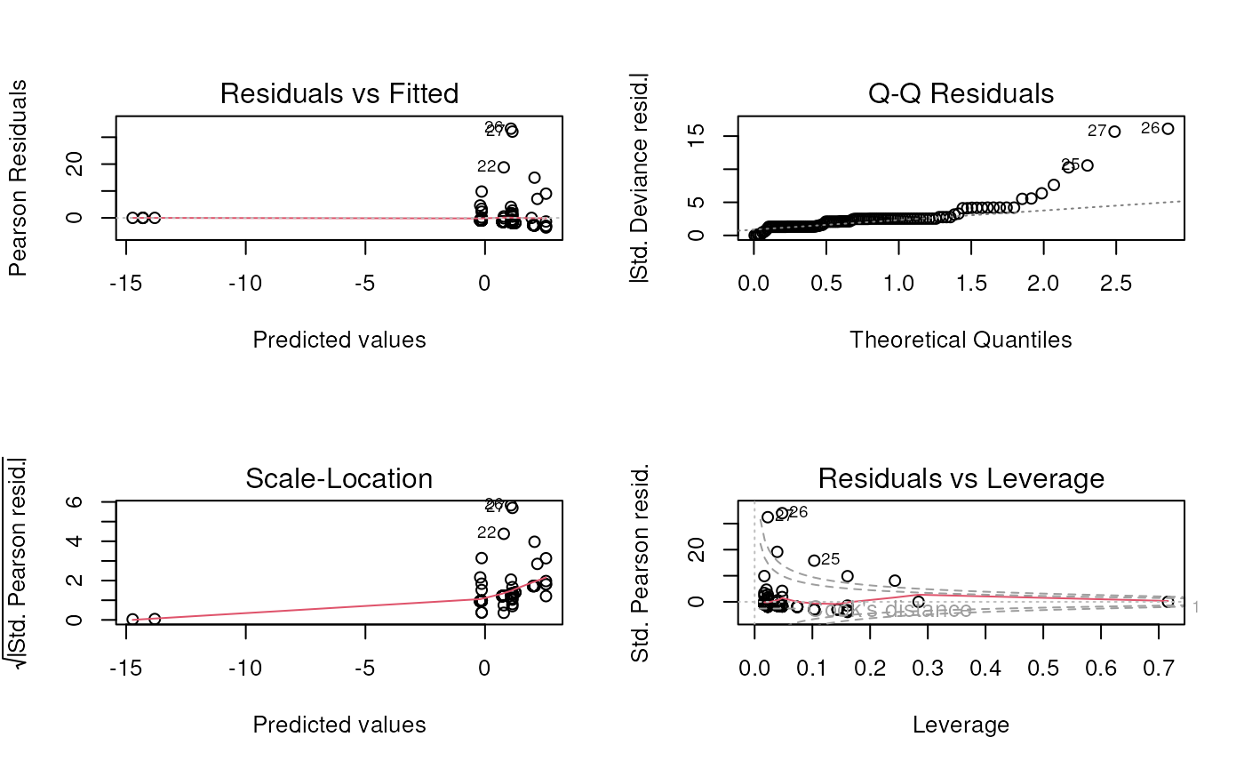
## Number of Fisher Scoring iterations: 12

Create and discuss Poisson model diagnostic plots

par(mfrow = c(2, 2))
plot(fit.pois)

## Warning: not plotting observations with leverage one:
##   17, 38, 72, 86

Levi Waldron