Session 1: Multiple linear regression review

Levi Waldron

Learning objectives and outline

Learning objectives

1. identify systematic and random components of a multiple linear regression model
2. define terminology used in a multiple linear regression model
3. define and explain the use of dummy variables
4. interpret multiple linear regression coefficients for continuous and categorical variables
5. use model formulae to multiple linear models
6. define and interpret interactions between variables
7. interpret ANOVA tables

Outline

1. multiple regression terminology and notation
2. continuous & categorical predictors
3. interactions
4. ANOVA tables
5. Model formulae

Multiple Linear Regression

Systematic part of model

For more detail: Vittinghoff section 4.2

$$E[y|x] = \beta_0 + \beta_1 x_1 + \beta_2 x_2 + ... + \beta_p x_p$$

• $E[y|x]$ is the expected value of $y$ given $x$
• $y$ is the outcome, response, or dependent variable
• $x$ is the vector of predictors / independent variables
• $x_p$ are the individual predictors or independent variables
• $\beta_p$ are the regression coefficients

Random part of model

$y_i = E[y_i|x_i] + \epsilon_i$

$y_i = \beta_0 + \beta_1 x_{1i} + \beta_2 x_{2i} + ... + \beta_p x_{pi} + \epsilon_i$

• $x_{ji}$ is the value of predictor $x_j$ for observation $i$

Assumption: $\epsilon_i \stackrel{iid}{\sim} N(0, \sigma_\epsilon^2)$

• Normal distribution
• Mean zero at every value of predictors
• Constant variance at every value of predictors
• Values that are statistically independent

Continuous predictors

• Coding: as-is, or may be scaled to unit variance (which results in adjusted regression coefficients)
• Interpretation for linear regression: An increase of one unit of the predictor results in this much difference in the continuous outcome variable
  • additive model

Binary predictors (2 levels)

• Coding: indicator or dummy variable (0-1 coding)
• Interpretation for linear regression: the increase or decrease in average outcome levels in the group coded “1”, compared to the reference category (“0”)
  • e.g. $E(y|x) = \beta_0 + \beta_1 x$
  • where x={ 1 if male, 0 if female }

Multilevel Categorical Predictors (Ordinal or Nominal)

• Coding: $K-1$ dummy variables for $K$-level categorical variables *
• Interpretation for linear regression: as above, the comparisons are done with respect to the reference category
• Testing significance of multilevel categorical predictor: partial F-test, a.k.a. nested ANOVA

* STATA and R code dummy variables automatically, behind-the-scenes

Inference from multiple linear regression

• Coefficients are t-distributed when assumptions are correct
• Variance in the estimates of each coefficient can be calculated
• The t-test of the null hypothesis $H_0: \beta_1 = 0$ and from confidence intervals tests whether $x_1$ predicts $y$, holding other predictors constant
  • often used in causal inference to control for confounding: see section 4.4

Interaction (effect modification)

How is interaction / effect modification modeled?

Interaction is modeled as the product of two covariates: $$E[y|x] = \beta_0 + \beta_1 x_1 + \beta_2 x_2 + \beta_{12} x_1*x_2$$

What is interaction / effect modification?

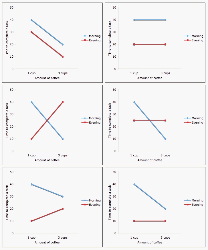
Interaction between coffee and time of day on performance

Image credit: http://personal.stevens.edu/~ysakamot/

Analysis of Variance

Review of the ANOVA table

Source of Variation	Sum Sq	Deg Fr	Mean Sq	F
Model	MSS	k	MSS/k	(MSS/k)/MSE
Residual	RSS	n-(k-1)	RSS/(n-k-1)
Total	TSS	n-1

• $k$ = Model degrees of freedom = coefficients - 1
• $n$ = Number of observations
• F is F-distributed with $k$ numerator and $n-(k-1)$ denominator degrees of freedom

Model formulae

What are model formulae?

Model formulae tutorial

• Model formulae are shortcuts to defining linear models in R
• Regression functions in R such as aov(), lm(), glm(), and coxph() all accept the “model formula” interface.
• The formula determines the model that will be built (and tested) by the R procedure. The basic format is:

response variable ~ explanatory variables

• The tilde means “is modeled by” or “is modeled as a function of.”

Model formula for simple linear regression

y ~ x

• where “x” is the explanatory (independent) variable
• “y” is the response (dependent) variable.

Model formula for multiple linear regression

Additional explanatory variables would be added as follows:

y ~ x + z

Note that “+” does not have its usual meaning, which would be achieved by:

y ~ I(x + z)

Types of standard linear models

lm( y ~ u + v)

u and v factors: ANOVA
u and v numeric: multiple regression
one factor, one numeric: ANCOVA

Model formulae cheatsheet

symbol	example	meaning
+	+ x	include this variable
-	- x	delete this variable
:	x : z	include the interaction
*	x * z	include these variables and their interactions
/	x / z	nesting: include z nested within x
|	x | z	conditioning: include x given z
^	(u + v + w)^3	include these variables and
		all interactions up to three way
1	-1	intercept: delete the intercept

Model formulae comprehension Q&A #1

How to interpret the following model formulae?

y ~ u + v + w + u:v + u:w + v:w
y ~ u * v * w - u:v:w
y ~ (u + v + w)^2

Model formulae comprehension Q&A #2

How to interpret the following model formulae?

y ~ u + v + w + u:v + u:w + v:w + u:v:w
y ~ u * v * w
y ~ (u + v + w)^3