Session 1 lab: Association between cholesterol and age

Learning objectives

Load a tab-separated dataset into R
Create a simple scatterplot using ggplot2
Fit and analyze a multiple linear regression model
Compare two nested models using a nested Analysis of Variance (partial F test)

Exercises

Load the cholesterol.tsv dataset into R
Fit linear models with age, state, and interaction terms as predictors
Compare a simple linear regression to a multiple linear regression using Analysis of Variance partial F-test
Use backwards selection from a full model with interactions to choose the best prediction model

Load the dataset

Figure out this command using File - Import Dataset

library(readr)
chol <- read_table("cholesterol.tsv", 
    col_types = cols(age = col_double()))
summary(chol)

##   cholesterol         age           state          
##  Min.   :112.0   Min.   :18.00   Length:30         
##  1st Qu.:181.2   1st Qu.:39.50   Class :character  
##  Median :199.0   Median :48.00   Mode  :character  
##  Mean   :213.7   Mean   :48.57                     
##  3rd Qu.:247.0   3rd Qu.:58.00                     
##  Max.   :356.0   Max.   :78.00

Create a scatterplot of Cholesterol vs. Age

Take Data Science Module 1 “Data Visualization Basics” first if you aren’t familiar with ggplot2:

library(ggplot2)
ggplot(chol, aes(x=age, y=cholesterol, shape=state, color=state)) + 
  geom_point(size=4) +
  geom_smooth(method=lm, se = FALSE)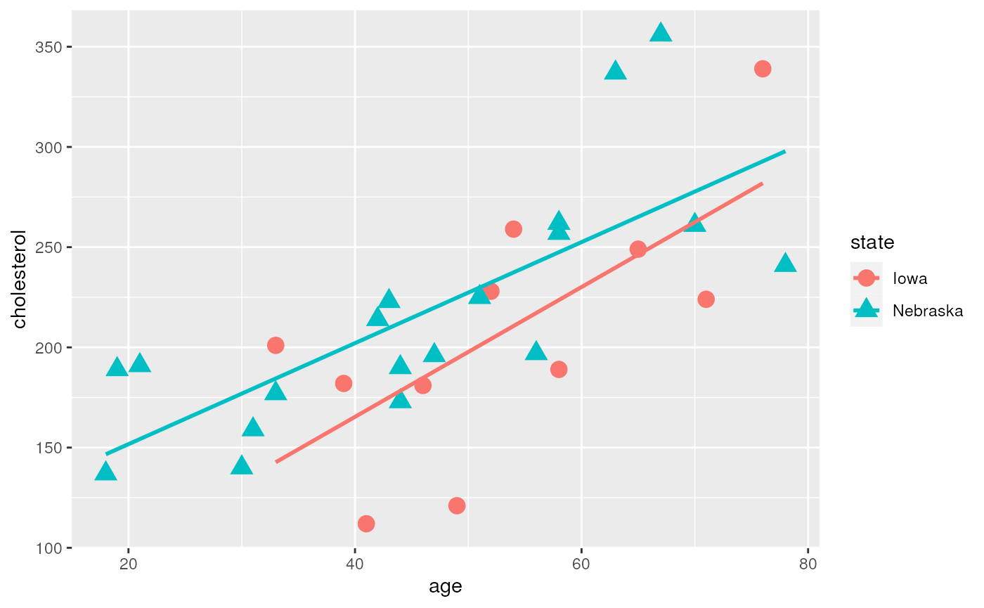

Fit a linear model with age, state, and interaction as predictors

cholesterol as the outcome variable.

fit <- lm(cholesterol ~ age * state, data=chol)
summary(fit)

## 
## Call:
## lm(formula = cholesterol ~ age * state, data = chol)
## 
## Residuals:
##     Min      1Q  Median      3Q     Max 
## -73.480 -31.907  -4.303  22.829  85.833 
## 
## Coefficients:
##                   Estimate Std. Error t value Pr(>|t|)   
## (Intercept)        35.8112    55.1166   0.650  0.52156   
## age                 3.2381     1.0088   3.210  0.00352 **
## stateNebraska      65.4866    61.9834   1.057  0.30045   
## age:stateNebraska  -0.7177     1.1628  -0.617  0.54247   
## ---
## Signif. codes:  0 '***' 0.001 '**' 0.01 '*' 0.05 '.' 0.1 ' ' 1
## 
## Residual standard error: 43.14 on 26 degrees of freedom
## Multiple R-squared:  0.5326, Adjusted R-squared:  0.4786 
## F-statistic: 9.875 on 3 and 26 DF,  p-value: 0.00016

Create an ANOVA table for this fit

anova(fit)

## Analysis of Variance Table
## 
## Response: cholesterol
##           Df Sum Sq Mean Sq F value    Pr(>F)    
## age        1  48976   48976 26.3124 2.388e-05 ***
## state      1   5456    5456  2.9315   0.09877 .  
## age:state  1    709     709  0.3809   0.54247    
## Residuals 26  48395    1861                      
## ---
## Signif. codes:  0 '***' 0.001 '**' 0.01 '*' 0.05 '.' 0.1 ' ' 1

Diagnostic plots for full model

par(mfrow=c(2, 2))
plot(fit)

Partial F-test for two models

fit1 <- lm(cholesterol ~ state, data=chol)
fit2 <- lm(cholesterol ~ state + age, data = chol)
anova(fit1, fit2)

## Analysis of Variance Table
## 
## Model 1: cholesterol ~ state
## Model 2: cholesterol ~ state + age
##   Res.Df    RSS Df Sum of Sq      F    Pr(>F)    
## 1     28 102924                                  
## 2     27  49104  1     53820 29.593 9.361e-06 ***
## ---
## Signif. codes:  0 '***' 0.001 '**' 0.01 '*' 0.05 '.' 0.1 ' ' 1

Backwards selection to select the best prediction model

library(MASS)
fit <- lm(cholesterol ~ age * state, data=chol)
step <- stepAIC(fit, direction = "backward")

## Start:  AIC=229.58
## cholesterol ~ age * state
## 
##             Df Sum of Sq   RSS    AIC
## - age:state  1    709.05 49104 228.01
## <none>                   48395 229.58
## 
## Step:  AIC=228.01
## cholesterol ~ age + state
## 
##         Df Sum of Sq    RSS    AIC
## <none>                49104 228.01
## - state  1      5456  54560 229.18
## - age    1     53820 102924 248.22

AIC = Akaike’s Information Criterion

Levi Waldron