Session 9 lab exercises: Repeated Measures and Longitudinal Analysis I

Learning objectives

Create and interpret a notched barplot
Create spaghetti / line plots for grouped data
Use pivot_wider to create a wide-format dataframe
Do a manual ICC calculation
Write a function
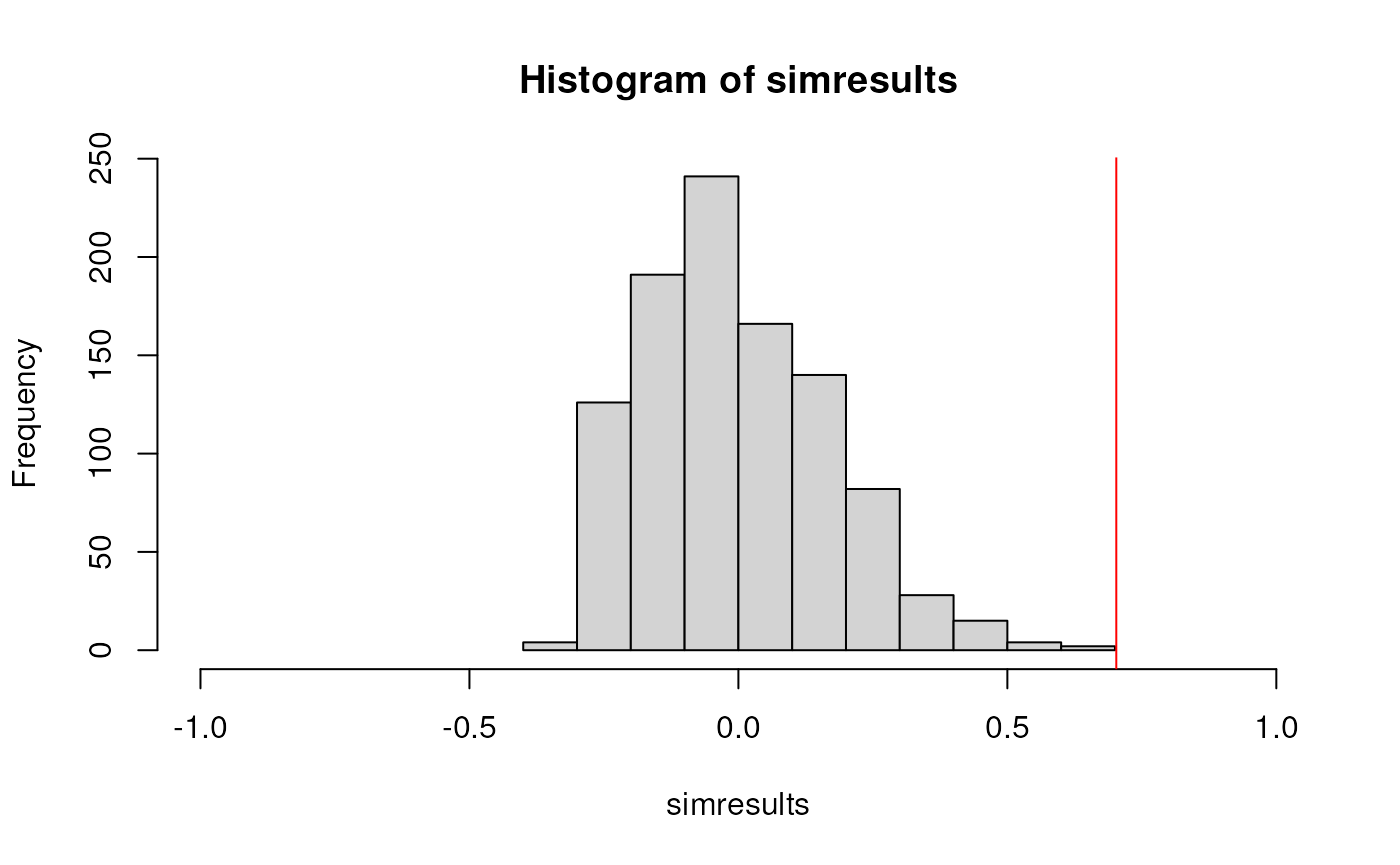
Perform a permutation simulation

Exercises

Read the fecal fat dataset and convert pilltype and subject to factors

library(readr)
library(dplyr)
dat <- read_csv("fecfat.csv") %>%
  mutate(pilltype = factor(pilltype, levels=c("none", "capsule", "tablet", "coated"))) %>%
  mutate(subject = factor(subject))

Create a notched boxplot of the data.

library(ggplot2)
ggplot(dat, aes(x = pilltype, y = fecfat)) +
  geom_boxplot(notch = TRUE, outlier.shape = NA) +
  geom_jitter(width = 0.2, alpha = 0.5) +
  theme_grey(base_size = 12) +
  theme(legend.position = "none")

## Notch went outside hinges
## ℹ Do you want `notch = FALSE`?
## Notch went outside hinges
## ℹ Do you want `notch = FALSE`?
## Notch went outside hinges
## ℹ Do you want `notch = FALSE`?
## Notch went outside hinges
## ℹ Do you want `notch = FALSE`?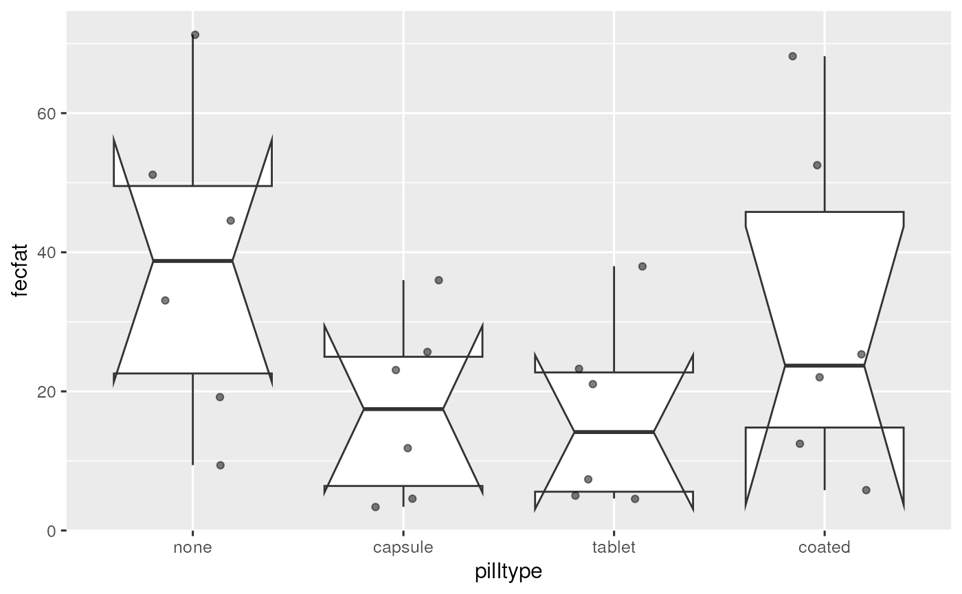

Interpret the notches. What is wrong with the usual interpretation in this example?

If the observations are independent (ie assumptions of a one-way AOV are met), notches can be used to visually perform a pairwise hypothesis test for difference of medians.

It’s wrong here because these are grouped / hierarchical data, and observations are not independent.

Subtract subject means from the fecal fat data, manually and using residuals of a one-way AOV

dat <- dat %>% group_by(subject) %>% 
  mutate(fecfatminusmean = fecfat - mean(fecfat)) %>%
  ungroup() %>%
  mutate(fecfatminusmean2 = residuals(lm(fecfat ~ subject, data = .)))

Make line plots for each subject, with and without subject mean centering

p1 <- ggplot(dat, aes(x = pilltype, y = fecfat, group = subject, lty = subject)) +
  geom_line() +
  labs(subtitle = "Raw data") +
  theme(axis.text.x = element_text(angle = 45, vjust = 1, hjust=1)) +
  xlab("Treatment") + ylab("Fecal Fat (mg/day)") +
  theme(legend.position = "none")
p2 <- ggplot(dat, aes(x = pilltype, y = fecfatminusmean, group = subject, lty = subject)) +
  geom_line() +
  labs(subtitle = "Subject means subtracted") +
  theme(axis.text.x = element_text(angle = 45, vjust = 1, hjust=1)) +
  xlab("Treatment") + ylab("Fecal Fat (mg/day)")
library(gridExtra)

## 
## Attaching package: 'gridExtra'

## The following object is masked from 'package:dplyr':
## 
##     combine

grid.arrange(p1, p2, ncol=2, respect=TRUE)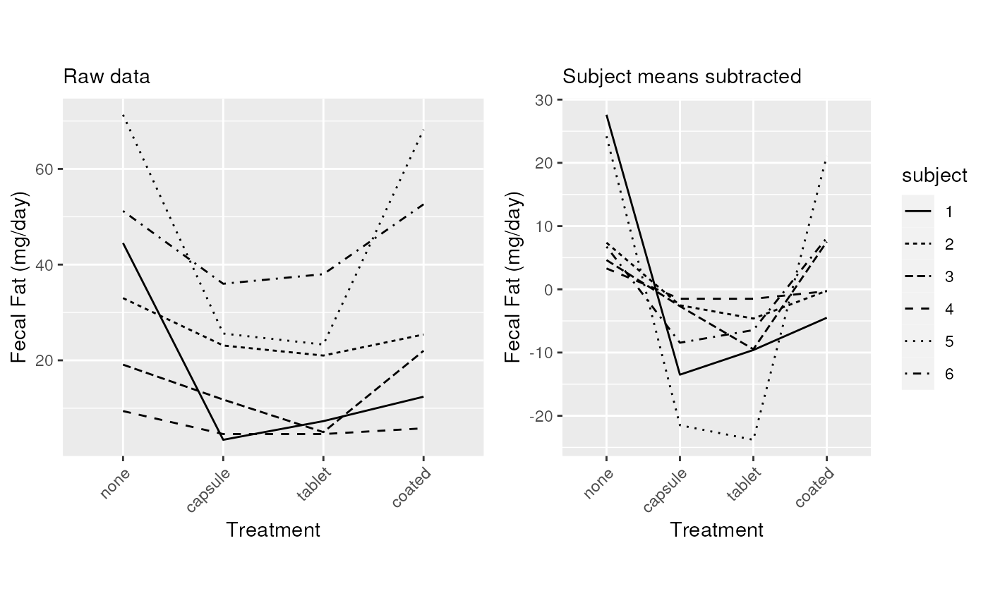

Convert to a wide-format dataset and remove the subject column

library(tidyr)
dat %>%
  select(-starts_with("fecfatminus")) %>%
  pivot_wider(names_from =pilltype, values_from = fecfat) %>%
  select(-subject)

## # A tibble: 6 × 4
##    none tablet capsule coated
##   <dbl>  <dbl>   <dbl>  <dbl>
## 1 44.5    7.30    3.40  12.4 
## 2 33     21      23.1   25.4 
## 3 19.1    5      11.8   22   
## 4  9.40   4.60    4.60   5.80
## 5 71.3   23.3    25.6   68.2 
## 6 51.2   38      36     52.6

Write a function to calculate subject and residual variance and ICC of this dataset as a vector

ICCfun <- function(x) {
  fit2way <- lm(fecfat ~ subject + pilltype, data = x)
  subjvar_uncorrected <- x %>% group_by(subject) %>%
    summarize(MEAN = mean(fecfat), .groups = "drop") %>%
    pull(MEAN) %>%
    var()
  correction <- sum(residuals(fit2way) ^ 2) / 15 / 4
  subjvar <- subjvar_uncorrected - correction
  residualvar <- sum(residuals(fit2way) ^ 2) / 15
  ICC <- subjvar / (subjvar + residualvar)
  output <- c(subjvar, residualvar, ICC)
  names(output) <- c("subjectvar", "residualvar", "ICC")
  return(output)
}
ICCfun(dat)

##  subjectvar residualvar         ICC 
## 252.6692760 106.9988878   0.7025066

Create a simulated dataset where subjects are randomized for each treatment

set.seed(1)
datrand <- dat %>% 
  group_by(pilltype) %>%
  mutate(subject = sample(subject)) %>%
  arrange(subject)

compare ICC for your original and simulated dataset

ICCfun(dat)

##  subjectvar residualvar         ICC 
## 252.6692760 106.9988878   0.7025066

ICCfun(datrand)

##  subjectvar residualvar         ICC 
##  62.8746156 296.7935482   0.1748128

Repeat the simulation 999 times, and compare to your original dataset

simulateData <- function(x){
  x %>%
  group_by(pilltype) %>%
  mutate(subject = sample(subject)) %>%
  arrange(subject)
}

set.seed(1)
simresults <- replicate(n=999, ICCfun(simulateData(dat))[3])

hist(simresults, xlim = c(-1, 1))
abline(v = ICCfun(dat), col = "red")

sum(simresults > ICCfun(dat))

## [1] 0

Levi Waldron