Session 8: Survival analysis part 3

Learning objectives and outline

Learning objectives

Check model assumptions and fit of the Cox model
- residuals analysis
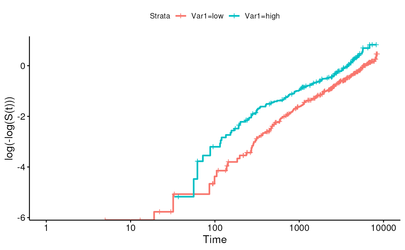
- log-minus-log plot
Fit and interpret multivariate Cox models
- perform tests for trend
- predict survival for specific covariate patterns
- predict survival for adjusted coefficients
Explain stratified analysis
Identify situations of competing risks
Describe the application of Propensity Score analysis

Vittinghoff sections 6.2-6.4

Outline

Review
Assumptions of Cox PH model
Tests for trend
Predictions for specific covariate patterns
Stratification
Competing risks
Propensity Score analysis to control for confounding

Review

Cox proportional hazards model

Cox proportional hazard regression assesses the relationship between a right-censored, time-to-event outcome and multiple predictors:
- categorical variables (e.g., treatment groups)
- continuous variables

\[ log(HR(x_i)) = log \frac{h(t|x_i)}{h_0(t)} = \beta_0 + \beta_1 x_{1i} + \beta_2 x_{2i} + ... + \beta_p x_{pi} \]

\(HR(x_i)\) is the hazard of patient \(i\) relative to baseline
\(h(t|x_i)\) is the time-dependent hazard function \(h(t)\) for patient \(i\)
\(h_0(t)\) is the baseline hazard function, and is the negative of the slope of the \(S_0(t)\), the baseline survival function.
Multiplicative model

Caveats and Assumptions

Categories with no events
- can occur when the group is small or its risk is low
- HRs with respect to such a reference group are infinite
- hypothesis tests and CIs are difficult / impossible to interpret
Assumptions of Cox PH model
- Constant hazard ratio over time (proportional hazards)
- Linear association between log(HR) and predictors (log-linearity) / multiplicative relationship between hazard and predictors
- Independence of survival times between individuals in the sample
- Uninformative censoring: a censored participant is the same as an uncensored participant with the same covariates at still in the risk set after that time

Checking assumptions of Cox model

Residuals analysis

Residuals are used to investigate the lack of fit of a model to a given subject.
For Cox regression, there’s no easy analog to the usual “observed minus predicted” residual

suppressPackageStartupMessages(library(pensim))
set.seed(1)
mydat <- create.data(
  nvars = c(1, 1),
  nsamples = 500,
  cors = c(0, 0),
  associations = c(0.5, 0.5),
  firstonly = c(TRUE, TRUE),
  censoring = c(0, 8.5)
)$data

Rename variables of simulated data, and make one variable categorical:

suppressPackageStartupMessages(library(dplyr))
mydat <- mydat %>% rename(Var1 = a.1, Var2 = b.1) %>%
  mutate(Var1 = cut(Var1,
                    breaks = 2,
                    labels = c("low", "high")),
         time = ceiling(time * 1000))

Simulated data to test residuals methods

summary(mydat)

##    Var1          Var2               time           cens      
##  low :323   Min.   :-2.99695   Min.   :   5   Min.   :0.000  
##  high:177   1st Qu.:-0.79008   1st Qu.: 691   1st Qu.:0.000  
##             Median :-0.02126   Median :1970   Median :1.000  
##             Mean   :-0.04594   Mean   :2529   Mean   :0.526  
##             3rd Qu.: 0.68933   3rd Qu.:3874   3rd Qu.:1.000  
##             Max.   : 3.05574   Max.   :8481   Max.   :1.000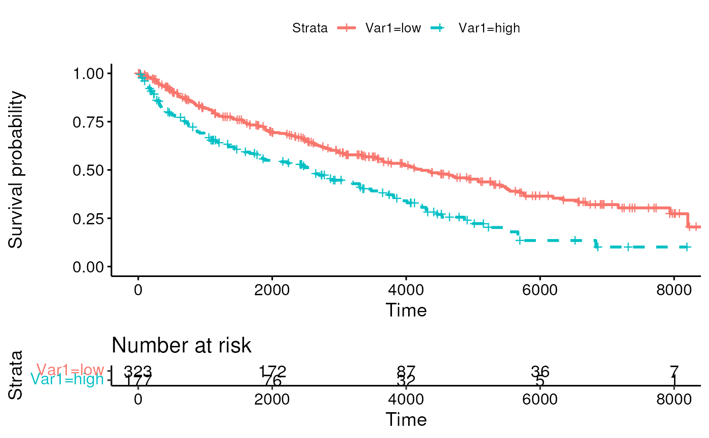

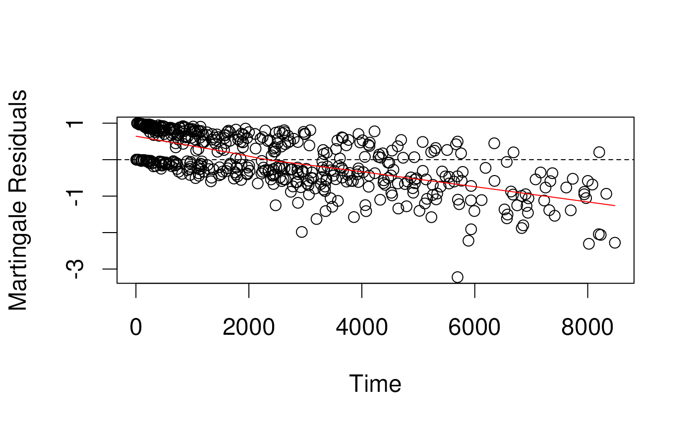
Kaplan-Meier plot of simulated data, stratified by Var1

Martingale residuals

censoring variable \(c_i\) (1 if event, 0 if censored) minus the estimated cumulative hazard function \(H(t_i, X_i, \beta_i)\) (1 - survival function)
- E.g., for a subject censored at 1 year (\(c_i=0\)), whose predicted cumulative hazard at 1 year was 30%, Martingale = \(0 - 0.30 = -0.30\).
- E.g. for a subject who had an event at 6 months, and whose predicted cumulative hazard at 6 months was 80%, Margingale = \(1 - 0.8 = 0.2\).
Problem: not symmetrically distributed, even when model fits the data well

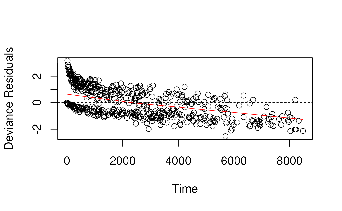
Martingale residuals in simulated data

Deviance residuals in simulated data

Deviance residuals are scaled Martingale residuals
Should be more symmetrically distributed about zero?
Observations with large deviance residuals are poorly predicted by the model

Schoenfeld residuals

technical definition: contribution of a covariate at each event time to the partial derivative of the log-likelihood
intuitive interpretation: the observed minus the expected values of the covariates at each event time.
a random (unsystematic) pattern across event times gives evidence the covariate effect is not changing with respect to time
If it is systematic, it suggests that as time passes, the covariate effect is changing.

Schoenfeld residuals for simulated data

Schoenfeld test for proportional hazards

Tests correlation between scaled Schoenfeld residuals and time
Equivalent to fitting a simple linear regression model with time as the predictor and residuals as the outcome
Parametric analog of smoothing the residuals against time using LOWESS
If the hazard ratio is constant, correlation should be zero.
- Positive values of the correlation suggest that the log-hazard ratio increases with time.

##          chisq df     p
## Var1   0.00887  1 0.925
## Var2   4.92734  1 0.026
## GLOBAL 5.07415  2 0.079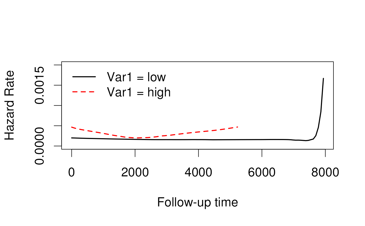

The hazard function h(t), stratified by Var1

Log-minus-log plot

Used to check proportional hazards assumption

Example: Primary Biliary Cirrhosis (PBC)

Mayo Clinic trial in primary biliary cirrhosis (PBC) of the liver conducted between 1974 and 1984, n=424 patients.
randomized placebo controlled trial of the drug D-penicillamine.
- 312 cases from RCT, plus additional 112 not from RCT.
Primary outcome is (censored) time to death

Kaplan-Meier plot of treatment and placebo arms

Tests for trend

What are tests for trend?

For models including an ordinal variablepush
Such as PBC stage (1, 2, 3, 4), age category, …
- Is there a linear / quadratic / cubic relationship between coefficients and their order?
- Test by LRT or Wald Test

Fitting a test for trend in R

Just define stage as an ordered factor and tests for trend are done automatically:

pbc.os <-
  mutate(pbc.os, stageordered = factor(stage, ordered = TRUE))
fit <- coxph(Surv(time, os) ~ stageordered, data = pbc.os)
summary(fit)

## Call:
## coxph(formula = Surv(time, os) ~ stageordered, data = pbc.os)
## 
##   n= 312, number of events= 125 
## 
##                   coef exp(coef) se(coef)      z Pr(>|z|)   
## stageordered.L  2.1759    8.8099   0.6801  3.199  0.00138 **
## stageordered.Q -0.3469    0.7069   0.5248 -0.661  0.50867   
## stageordered.C  0.3209    1.3784   0.2990  1.073  0.28316   
## ---
## Signif. codes:  0 '***' 0.001 '**' 0.01 '*' 0.05 '.' 0.1 ' ' 1
## 
##                exp(coef) exp(-coef) lower .95 upper .95
## stageordered.L    8.8099     0.1135    2.3231    33.410
## stageordered.Q    0.7069     1.4146    0.2527     1.977
## stageordered.C    1.3784     0.7255    0.7671     2.477
## 
## Concordance= 0.702  (se = 0.022 )
## Likelihood ratio test= 52.74  on 3 df,   p=2e-11
## Wald test            = 43.92  on 3 df,   p=2e-09
## Score (logrank) test = 53.85  on 3 df,   p=1e-11

Highly significant tests of overall fit by LRT, Wald, and logrank test.

Predictions for specific covariate patterns

How to predict survival from a Cox model?

The Cox model is a relative risk model
- only predicts relative risks between pairs of subjects
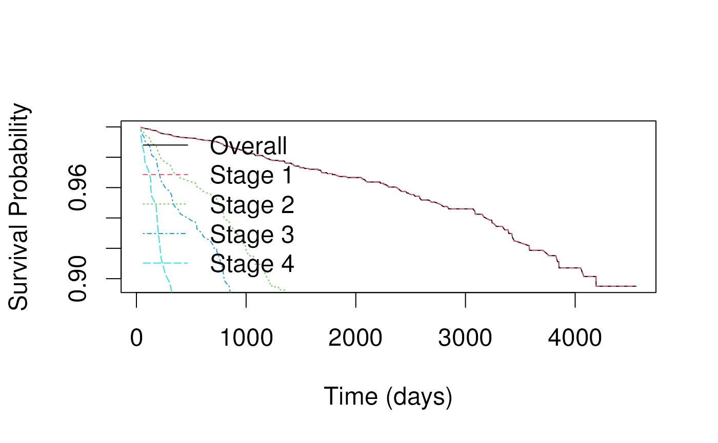
Key is to calculate the overall \(S(t)\), then multiply it by the relative hazard for the specific covariate pattern.
In this example we plot the baseline survival for all stages together, then for stages 1-4 separately.

Predicted survival for specific covariate patterns

Multivariate regression

Same coding and objectives as for lm() and glm()
- controlling for confounding
- testing for mediation
- testing for interaction

fit <- coxph(Surv(time, os) ~ age + sex + edema
             + stage + arm, data = pbc.os)
summary(fit)

## Call:
## coxph(formula = Surv(time, os) ~ age + sex + edema + stage + 
##     arm, data = pbc.os)
## 
##   n= 312, number of events= 125 
## 
##                   coef exp(coef)  se(coef)      z Pr(>|z|)    
## age           0.027618  1.028003  0.009362  2.950  0.00318 ** 
## sexf         -0.317540  0.727938  0.248839 -1.276  0.20193    
## edema0.5      0.538715  1.713804  0.275287  1.957  0.05036 .  
## edema1        2.080422  8.007845  0.276959  7.512 5.84e-14 ***
## stage2        1.535263  4.642546  1.034854  1.484  0.13793    
## stage3        1.998217  7.375893  1.016097  1.967  0.04923 *  
## stage4        2.666263 14.386101  1.016234  2.624  0.00870 ** 
## armtreatment  0.057946  1.059658  0.189200  0.306  0.75940    
## ---
## Signif. codes:  0 '***' 0.001 '**' 0.01 '*' 0.05 '.' 0.1 ' ' 1
## 
##              exp(coef) exp(-coef) lower .95 upper .95
## age             1.0280    0.97276    1.0093     1.047
## sexf            0.7279    1.37374    0.4470     1.186
## edema0.5        1.7138    0.58350    0.9992     2.940
## edema1          8.0078    0.12488    4.6534    13.780
## stage2          4.6425    0.21540    0.6108    35.288
## stage3          7.3759    0.13558    1.0067    54.040
## stage4         14.3861    0.06951    1.9630   105.430
## armtreatment    1.0597    0.94370    0.7313     1.535
## 
## Concordance= 0.77  (se = 0.022 )
## Likelihood ratio test= 107.6  on 8 df,   p=<2e-16
## Wald test            = 120.8  on 8 df,   p=<2e-16
## Score (logrank) test = 177.1  on 8 df,   p=<2e-16

Predicted survival for adjusted coefficients

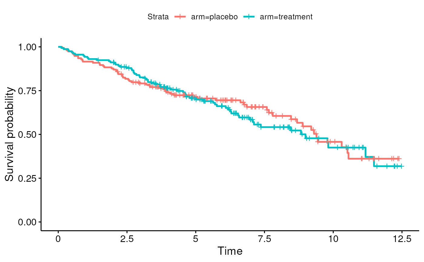
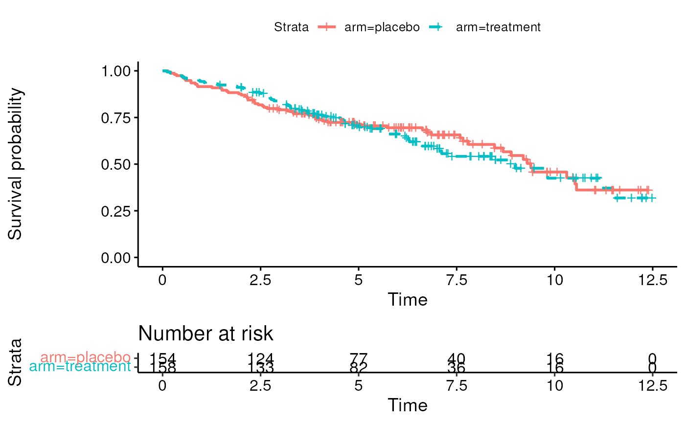
Can create Kaplan-Meier curves for crude or unadjusted coefficients
- Section 6.3.2.3 in Vittinghoff
Idea is to estimate hazard ratio in an unadjusted model:

unadjfit <- coxph(Surv(time, os) ~ stage, data = pbc.os)
coef(unadjfit)

##   stage2   stage3   stage4 
## 1.607014 2.149500 3.062775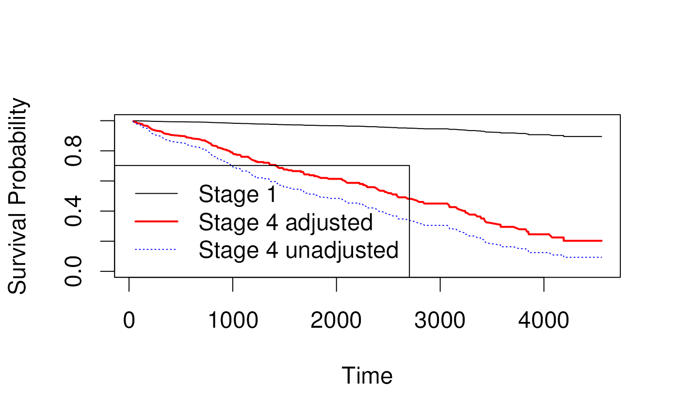

Predicted survival for adjusted coefficients (cont’d)

and in an adjusted model:

adjfit <- coxph(Surv(time, os) ~ age + sex + edema
                + stage + arm, data = pbc.os)
coef(adjfit)

##          age         sexf     edema0.5       edema1       stage2       stage3 
##    0.0276179   -0.3175396    0.5387152    2.0804217    1.5352629    1.9982170 
##       stage4 armtreatment 
##    2.6662626    0.0579460

Predicted survival for adjusted coefficients (cont’d)

The survival function will be calculated for a “baseline” group, say stage 1, then exponentiated with the adjusted coefficient, e.g.: \[ [S_{stage=1}(t)]^{exp(\beta_{stage=4})} \]

Stratification

What is stratification?

relevant to all kinds of regression, not just survival analysis
when analysis is separated into groups or strata
- must have an adequate number of events in each stratum (at least 5 to 7)
- can be used to adjust for variables with strong impact on survival
- can help solve proportional hazards violations
Strata have different baseline hazards
Coefficients / Hazard Ratios are calculated within stratum then combined.
Vittinghoff 6.3.2

How to stratify

Example - in R, strata() can be added to any model formula

mycox <- coxph(Surv(time, os) ~ trt + strata(stage), 
               data = pbc.os)
summary(mycox)

## Call:
## coxph(formula = Surv(time, os) ~ trt + strata(stage), data = pbc.os)
## 
##   n= 312, number of events= 125 
## 
##        coef exp(coef) se(coef)      z Pr(>|z|)
## trt -0.1063    0.8992   0.1814 -0.586    0.558
## 
##     exp(coef) exp(-coef) lower .95 upper .95
## trt    0.8992      1.112    0.6302     1.283
## 
## Concordance= 0.494  (se = 0.025 )
## Likelihood ratio test= 0.34  on 1 df,   p=0.6
## Wald test            = 0.34  on 1 df,   p=0.6
## Score (logrank) test = 0.34  on 1 df,   p=0.6

Competing Risks Data

What are competing risks?

Example from Vittinghoff 6.5: The MrOS study (Orwoll et al. 2005) followed men over 65 to examine predictors of bone fracture and low BMD (subclinical bone loss)
At end of study participants had:
- developed fracture (outcome of interest),
- remained alive without fracture (incomplete follow-up), or
- died prior to fracture (incomplete follow-up)

Orwoll, E. et al. (2005). Design and baseline characteristics of the osteoporotic fractures in men (MrOS) study–a large observational study of the determinants of fracture in older men. Contemporary Clinical Trials, 26(5), 569–585.

Why not treat died prior to fracture and alive without fracture as censored?

Recall the independent censoring assumption (Vittinghoff 6.6.4):
- censored people are similar to those who remain at risk in terms of developing the event of interest;
- censoring is independent of the event of interest.
- For patients who died this assumption is highly suspect

Reasons for right censored data

Cut-off date of analysis (administrative censoring):
- Censoring usually independent
Loss to follow-up
- Independence may be problematic if sicker individuals discontinue participant in study (lack of energy, too ill, return to home country)
- or if healthier individuals discontinue participation (don’t feel the need to continue, start new life in other country)
Competing risks:
- Often informative.
- In competing risks analysis, independence between competing risks is not required

Very brief summary of competing risk methods

1-to-1 mapping between hazard and cumulative incidence function is lost in competing risks
Standard Kaplan-Meier estimator is biased for competing risks data
- Aalen-Johansen estimator is better choice
Gary’s test is analogous to log-rank test
cause-specific standard Cox PH model might be useful for prognostic (causal) testing, but not estimating a population Hazard Ratio

Resources for competing risk methods

Z. Zhang, Survival analysis in the presence of competing risks, Ann Transl Med. 2017 Feb; 5(3): 47. PMID: 28251126
cmprsk package
riskRegression package

Propensity score analysis

What is propensity score analysis?

an alternative to multivariate regression to control for hypothesized confounders in observational studies:

outcome ~ exposure + counfounder1 + confounder2

a stratification approach that is more practical than stratifying on multiple hypothesized confounders
an approach to summarizing many covariates into a single score
a convenient approach to controlling for many hypothesized confounders

Propensity score approach to correction for confounders

Step 1: fit the propensity score model (no outcome) that predicts propensity for exposure based on confounders:

exposure ~ counfounder1 + confounder2

Step 2: use propensity predictions to match or stratify participants with similar propensity (for example, stratifying on quintiles of propensity)
Step 3: check adequacy of matching or stratification, ie by comparing attributes of matched participants
Step 4: test hypothesis among matched participants:

outcome ~ exposure

Propensity score references

P.C. Austin (2011), An Introduction to Propensity Score Methods for Reducing the Effects of Confounding in Observational Studies. Multivariate Behavioral Research, 46:3, 399-424, DOI: 10.1080/00273171.2011.568786
R. d’Agostino (1998), Tutorial in Biostatistics: propensity score methods for bias reduction in the comparison of a treatment to a non-randomized control group. Stat. Med. 17, 2265-2281. http://www.stat.ubc.ca/~john/papers/DAgostinoSIM1998.pdf
You don’t need any special package to do basic propensity score matching (e.g. stratifying by quintiles), but the MatchIt package provides multiple matching approaches, diagnostics, good documentation

Levi Waldron

Learning objectives and outline

Learning objectives

Outline

Review

Cox proportional hazards model

Caveats and Assumptions

Checking assumptions of Cox model

Residuals analysis

Simulated data to test residuals methods

Kaplan-Meier plot of simulated data, stratified by Var1

Martingale residuals

Martingale residuals in simulated data

Deviance residuals in simulated data

Schoenfeld residuals

Schoenfeld residuals for simulated data

Schoenfeld test for proportional hazards

The hazard function h(t), stratified by Var1

Log-minus-log plot

Example: Primary Biliary Cirrhosis (PBC)

Kaplan-Meier plot of treatment and placebo arms

Tests for trend

What are tests for trend?

Fitting a test for trend in R

Predictions for specific covariate patterns

How to predict survival from a Cox model?

Predicted survival for specific covariate patterns

Multivariate regression

Predicted survival for adjusted coefficients

Predicted survival for adjusted coefficients (cont’d)

Predicted survival for adjusted coefficients (cont’d)

Stratification

What is stratification?

How to stratify

Competing Risks Data

What are competing risks?

Why not treat died prior to fracture and alive without fracture as censored?

Reasons for right censored data

Very brief summary of competing risk methods

Resources for competing risk methods

Propensity score analysis

What is propensity score analysis?

Propensity score approach to correction for confounders

Propensity score references