Session 7: Survival Analysis 2
Levi Waldron
session_lecture.RmdLearning objectives and outline
Learning objectives
- Define proportional hazards
- Perform and interpret Cox proportional hazards regression
- Define time-dependent covariates and their use
- Identify the differences between parametric and semi-parametric survival models
- Identify situations when a parametric survival model might be useful
Review of survival and hazard functions
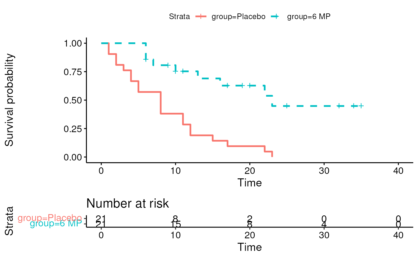
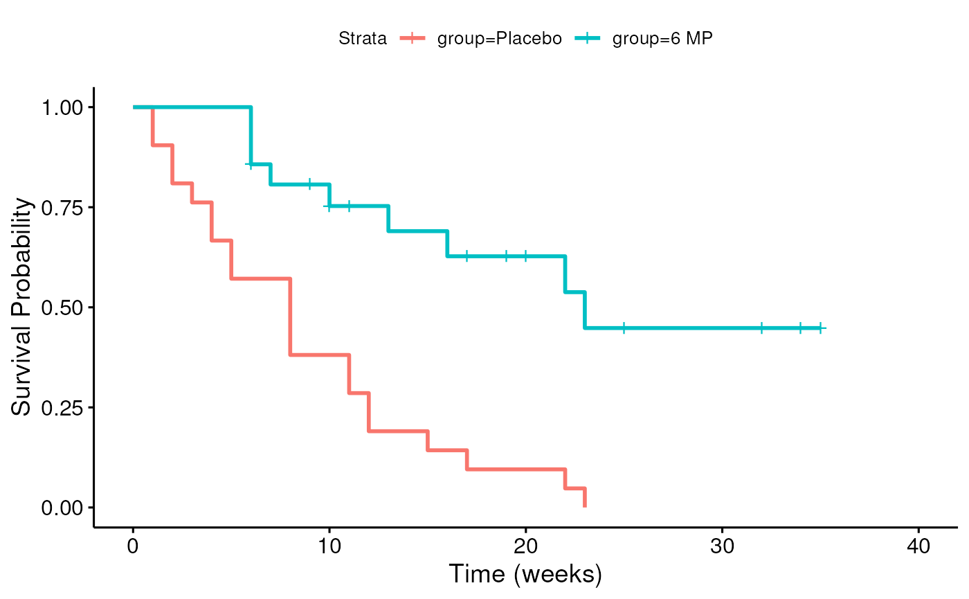
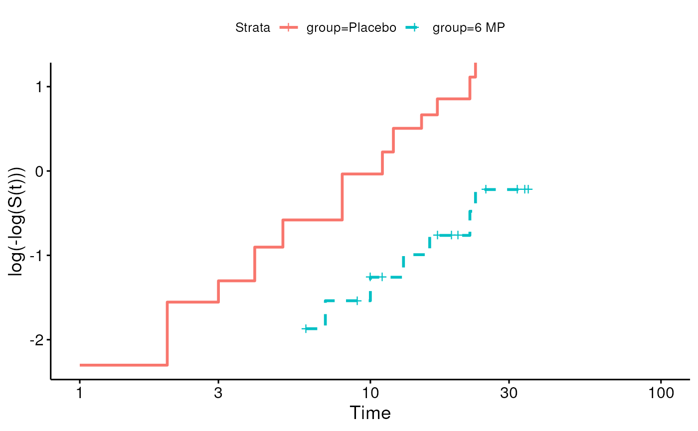
Recall leukemia Example
- Study of 6-mercaptopurine (6-MP) maintenance therapy for children in remission from acute lymphoblastic leukemia (ALL)
- 42 patients achieved remission from induction therapy and were then randomized in equal numbers to 6-MP or placebo.
- Survival time studied was from randomization until relapse.
Leukemia follow-up table
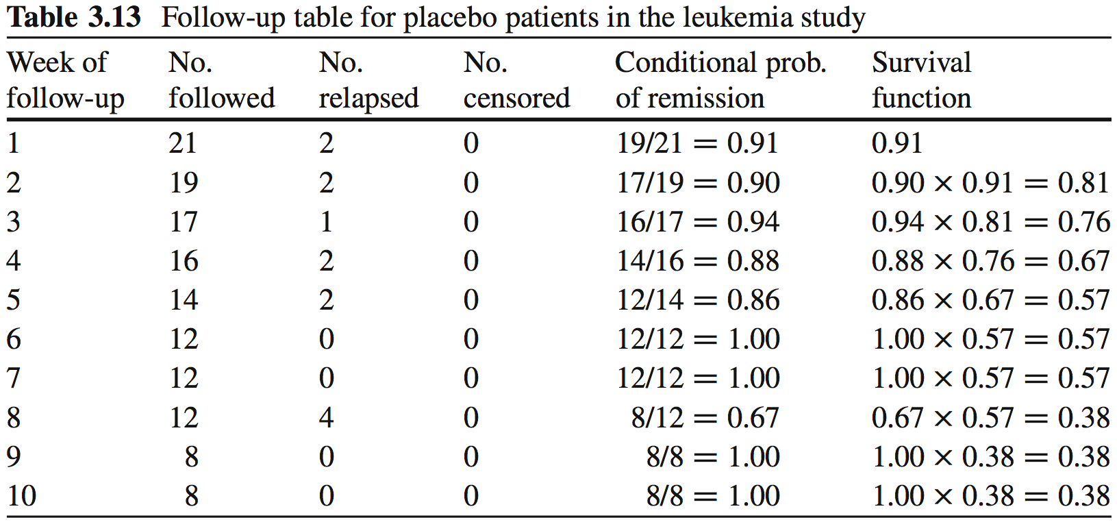
This is the Kaplan-Meier Estimate of the Survival function .
The hazard function h(t)
Definition: The survival function at time t, denoted , is the probability of being event-free at t. Equivalently, it is the probability that the survival time is greater than t.
Definition: The cumulative event function at time t, denoted , is the probability that the event has occurred by time t, or equivalently, the probability that the survival time is less than or equal to t. .
-
Definition: The hazard function is the short-term event rate for subjects who have not yet experienced an event.
- is the probability of an event in the time interval (s is small), given that the individual has survived up to time t

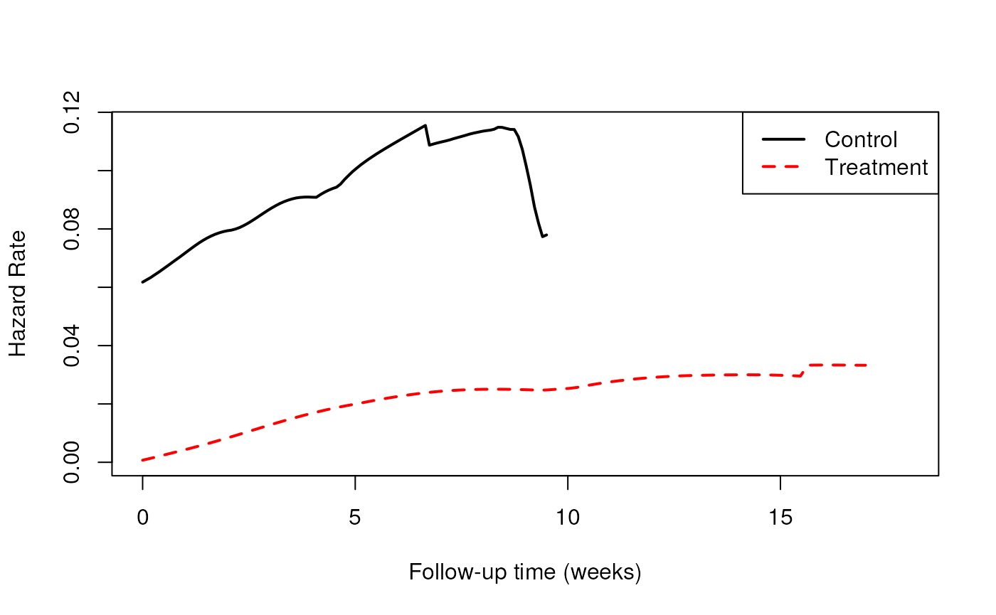
The Hazard Ratio (HR)
- If we are comparing the hazards of a control and a treatment group,
it could in general be a function of time:
- Interpretation: the risk of event for the treatment group compared to the control group, as a function of time
The Proportional Hazards Assumption
Definition: Under the proportional hazards assumption, the hazard ratio does not vary with time. That is, .
-
In other words, does not vary with time
- is a constant, , at all times t
- this assumption is about the population, of course there will be sampling variation

Cox proportional hazards model
Cox proportional hazards model
- Cox proportional hazards regression assesses relationship between a
right-censored, time-to-event outcome and predictors:
- categorical variables (e.g., treatment groups)
- continuous variables
- is the hazard of patient relative to baseline
- is the time-dependent hazard function for patient
- is the baseline hazard function
Multiplicative or additive model?
Interpretation of coefficients
- Coefficients
for a categorical / binary predictor:
- is the of the ratio of hazards for the comparison group relative to reference group ()
- Coefficients
for a continuous predictor:
- is the of the ratio of hazards for someone having a one unit higher value of (1 year, 1mm Hg, etc)
- If the hazard ratio () is close to 1 then the predictor does not affect survival
- If the hazard ratio is less than 1 then the predictor is protective (associated with improved survival)
- If the hazard ratio is greater than 1 then the predictor is associated with increased risk (= decreased survival)
Hypothesis testing and CIs
- Wald Test or Likelihood Ratio Test for coefficients
- equivalent to
- CIs typically obtained from Wald Test, reported for
Cox PH regression for Leukemia dataset
## Call:
## coxph(formula = Surv(time, cens) ~ group, data = leuk)
##
##   n= 42, number of events= 30
##
##              coef exp(coef) se(coef)      z Pr(>|z|)
## group6 MP -1.5721    0.2076   0.4124 -3.812 0.000138 ***
## ---
## Signif. codes:  0 '***' 0.001 '**' 0.01 '*' 0.05 '.' 0.1 ' ' 1
##
##           exp(coef) exp(-coef) lower .95 upper .95
## group6 MP    0.2076      4.817   0.09251    0.4659
##
## Concordance= 0.69  (se = 0.041 )
## Likelihood ratio test= 16.35  on 1 df,   p=5e-05
## Wald test            = 14.53  on 1 df,   p=1e-04
## Score (logrank) test = 17.25  on 1 df,   p=3e-05
Cox PH is a semi-parametric model
- Cox proportional hazards model is semi-parametric:
- assumes proportional hazards (PH), but no assumption on
- robust if PH assumption is not violated
- time-dependent covariates may resolve apparent violations of the PH assumption.
Summary: proportional hazards assumption
- Constant hazard ratio between groups over time (proportional hazards)
- A linear association between the natural log of the relative hazard
and the predictors (log-linearity)
- A multiplicative relationship between the predictors and the hazard
- Uninformative censoring
What to do when proportional hazards doesn’t hold?
- Time-dependent covariates
- Definition: A time-dependent covariate is a predictor whose values may vary with time.
-
Basic rule: You cannot look into the future in your
analysis (even though it took place in the past) E.g.:
- breast cancer chemotherapy patients divided into groups based on how much of the planned dose they received
- patients divided into groups based on early response to treatment (shrinkage of tumor, lowering of cholesterol, etc)
- interpolation of the values of a laboratory test linearly between observation times
- removing subjects who do not finish the treatment plan
- imputing the date of an adverse event as midway between observation times
Source: Using Time Dependent Covariates and Time Dependent Coefficients in the Cox Model
Immortal time bias example
- Immortal time bias is an example of looking into the future.
- E.g. Yee et al. reported that new statin users reported a
26% reduction in the risk of diabetes progression with one year or more
of treatment relative to never-users (adjusted HR 0.74, 95% CI: 0.56 to
0.97).
- New users excludes those who had received a lipid lowering drug from three years before to six months after cohort entry
- HR>1 was expected:people whose diabetes progresses are more likely to develop cardiovascular disease, an indication for statins.
- This is a result of an analysis error. Why?
- Yee et al. Statin use in type 2 diabetes mellitus is associated with a delay in starting insulin (http://onlinelibrary.wiley.com/doi/10.1111/j.1464-5491.2004.01263.x/full)
Immortal time bias example (cont’d)
- What was the analysis error?
- “new statin user” group was defined based on future initiation: knowledge unknown at the time of entry into the study
- guaranteed no events for statin users from cohort entry to start of statin use
- thus all persons in the treated group are “immortal” from time 0 until the initiation of statin treatment
- this period of immortality made treatment look more effective
Parametric survival models
What are “parametric” survival models?
- “Parametric” models estimate additional parameters for the
baseline hazard, e.g.:
- Weibull: hazard function is a polynomial
- exponential: hazard function is constant over time, survival function is exponential (special case of Weibull): e.g. healthy population with randomly occurring events
- many other options for assumption of distributions
- In most common implementation a log-transform of the time variable
is used
- then can be interpreted as Accelerated Failure Time (AFT) models.
Coefficients in parametric models
- The interpretation of
coefficients is different:
- Cox model:
- AFT models:
- The sign is opposite (i.e. if one is positive the other is negative)
Why use a parametric survival model?
- Can be more powerful if assumption is correct
- may help with small numbers of events
- Extra capabilities:
- smooth estimation of baseline hazard
- extrapolation
- complicated censoring
- Easy to interpret: coefficients are
- Easy to fit: replace
survival::coxphwithsurvival::survreg