Session 3: Regression coefficients and model matrices

Learning objectives and outline

Learning objectives

Interpret main effect coefficients in logistic regression
Interpret interaction terms in logistic regression
Define and interpret model matrices for (generalized) linear models

Outline

Review of GLM
Interpretation of logistic regression coefficients
Introduction to model matrices

GLM review

Components of GLM

Random component specifies the conditional distribution for the response variable
- doesn’t have to be normal
- can be any distribution in the “exponential” family of distributions
Systematic component specifies linear function of predictors (linear predictor)
Link [denoted by g(.)] specifies the relationship between the expected value of the random component and the systematic component
- can be linear or nonlinear

Logistic Regression as GLM

The model: \[ \begin{aligned} Logit(P(x)) &= log \left( \frac{P(x)}{1-P(x)} \right) \notag\\ &= \beta_0 + \beta_1 x_{1i} + \beta_2 x_{2i} + ... + \beta_p x_{pi} \notag \end{aligned} \]
Random component: \(y_i\) follows a Binomial distribution (outcome is a binary variable)
Systematic component: linear predictor \[ \beta_0 + \beta_1 x_{1i} + \beta_2 x_{2i} + ... + \beta_p x_{pi} \]
Link function: logit (log of the odds that the event occurs)

\[ g(P(x)) = logit(P(x)) = log\left( \frac{P(x)}{1-P(x)} \right) \]

\[ P(x) = g^{-1}\left( \beta_0 + \beta_1 x_{1i} + \beta_2 x_{2i} + ... + \beta_p x_{pi} \right) \]

Additive vs. multiplicative models

Linear regression is an additive model
- e.g. for two binary variables \(\beta_1 = 1.5\), \(\beta_2 = 1.5\).
- If \(x_1=1\) and \(x_2=1\), this adds 3.0 to \(E(y|x)\)
Logistic regression is a multiplicative model
- It is additive on log-odds scale
- If \(x_1=1\) and \(x_2=1\), this adds 3.0 to \(log(\frac{P}{1-P})\)
- Odds-ratio \(\frac{P}{1-P}\) increases 20-fold: \(exp(1.5+1.5)\) or \(exp(1.5) * exp(1.5)\)

Interpretation of main effects and interactions in logistic regression

Motivating example: contraceptive use data

From http://data.princeton.edu/wws509/datasets/#cuse

cuse <- read.table("cuse.dat", header=TRUE)
summary(cuse)

##      age             education          wantsMore            notUsing     
##  Length:16          Length:16          Length:16          Min.   :  8.00  
##  Class :character   Class :character   Class :character   1st Qu.: 31.00  
##  Mode  :character   Mode  :character   Mode  :character   Median : 56.50  
##                                                           Mean   : 68.75  
##                                                           3rd Qu.: 85.75  
##                                                           Max.   :212.00  
##      using      
##  Min.   : 4.00  
##  1st Qu.: 9.50  
##  Median :29.00  
##  Mean   :31.69  
##  3rd Qu.:49.00  
##  Max.   :80.00

Univariate regression on “wants more children”

fit <- glm(cbind(using, notUsing) ~ wantsMore, 
           data=cuse, family=binomial("logit"))
summary(fit)

## 
## Call:
## glm(formula = cbind(using, notUsing) ~ wantsMore, family = binomial("logit"), 
##     data = cuse)
## 
## Coefficients:
##              Estimate Std. Error z value Pr(>|z|)    
## (Intercept)  -0.18636    0.07971  -2.338   0.0194 *  
## wantsMoreyes -1.04863    0.11067  -9.475   <2e-16 ***
## ---
## Signif. codes:  0 '***' 0.001 '**' 0.01 '*' 0.05 '.' 0.1 ' ' 1
## 
## (Dispersion parameter for binomial family taken to be 1)
## 
##     Null deviance: 165.772  on 15  degrees of freedom
## Residual deviance:  74.098  on 14  degrees of freedom
## AIC: 149.61
## 
## Number of Fisher Scoring iterations: 4

Interpretation of “wants more children” table

Coefficients for (Intercept) and dummy variables
Coefficients are normally distributed when assumptions are correct

Interpretation of “wants more children” coefficients

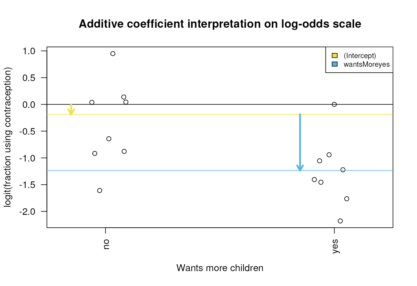
Diagram of the estimated coefficients in the GLM. The yellow arrow indicates the Intercept term, which goes from zero to the mean of the reference group (here the ‘wantsMore = no’ samples). The blue arrow indicates the difference in log-odds of the yes group minus the no group, which is negative in this example. The circles show the individual samples, jittered horizontally to avoid overplotting.

Regression on age

Four age groups
- three dummy variables age25-29, age30-39, age40-49
- how to interpret them?

Regression on age

fit <- glm(cbind(using, notUsing) ~ age, 
           data=cuse, family=binomial("logit"))
summary(fit)

## 
## Call:
## glm(formula = cbind(using, notUsing) ~ age, family = binomial("logit"), 
##     data = cuse)
## 
## Coefficients:
##             Estimate Std. Error z value Pr(>|z|)    
## (Intercept)  -1.5072     0.1303 -11.571  < 2e-16 ***
## age25-29      0.4607     0.1727   2.667  0.00765 ** 
## age30-39      1.0483     0.1544   6.788 1.14e-11 ***
## age40-49      1.4246     0.1940   7.345 2.06e-13 ***
## ---
## Signif. codes:  0 '***' 0.001 '**' 0.01 '*' 0.05 '.' 0.1 ' ' 1
## 
## (Dispersion parameter for binomial family taken to be 1)
## 
##     Null deviance: 165.772  on 15  degrees of freedom
## Residual deviance:  86.581  on 12  degrees of freedom
## AIC: 166.09
## 
## Number of Fisher Scoring iterations: 4

Recall model formulae

symbol	example	meaning
+	+ x	include this variable
-	- x	delete this variable
:	x : z	include the interaction
*	x * z	include these variables and their interactions
^	(u + v + w)^3	include these variables and all interactions up to three way
1	-1	intercept: delete the intercept

Regression on age and wantsMore

fit <- glm(cbind(using, notUsing) ~ age + wantsMore, 
           data=cuse, family=binomial("logit"))

	Estimate	Std. Error	z value	Pr(>\|z\|)
(Intercept)	-0.87	0.16	-5.54	0.00
age25-29	0.37	0.18	2.10	0.04
age30-39	0.81	0.16	5.06	0.00
age40-49	1.02	0.20	5.01	0.00
wantsMoreyes	-0.82	0.12	-7.04	0.00

Interaction / Effect Modification

What if we want to know whether the effect of age is modified by whether the woman wants more children or not?

Interaction is modeled as the product of two covariates: \[ E[y|x] = \beta_0 + \beta_1 x_1 + \beta_2 x_2 + \beta_{12} x_1*x_2 \]

Interaction / Effect Modification (fit)

fit <- glm(cbind(using, notUsing) ~ age * wantsMore, 
           data=cuse, family=binomial("logit"))

	Estimate	Std. Error	z value	Pr(>\|z\|)
(Intercept)	-1.46	0.30	-4.90	0.00
age25-29	0.64	0.36	1.78	0.07
age30-39	1.54	0.32	4.84	0.00
age40-49	1.76	0.34	5.14	0.00
wantsMoreyes	-0.06	0.33	-0.19	0.85
age25-29:wantsMoreyes	-0.27	0.41	-0.65	0.51
age30-39:wantsMoreyes	-1.09	0.37	-2.92	0.00
age40-49:wantsMoreyes	-1.37	0.48	-2.83	0.00

The Design Matrix

What is the design matrix, and why?

What? The design matrix is the most generic, flexible way to specify them
Why? There are multiple possible and reasonable regression models for a given study design.

Matrix notation for the multiple linear regression model

\[ \, \begin{pmatrix} Y_1\\ Y_2\\ \vdots\\ Y_N \end{pmatrix} = \begin{pmatrix} 1&x_1\\ 1&x_2\\ \vdots\\ 1&x_N \end{pmatrix} \begin{pmatrix} \beta_0\\ \beta_1 \end{pmatrix} + \begin{pmatrix} \varepsilon_1\\ \varepsilon_2\\ \vdots\\ \varepsilon_N \end{pmatrix} \]

or simply:

\[ \mathbf{Y}=\mathbf{X}\boldsymbol{\beta}+\boldsymbol{\varepsilon} \]

The design matrix is \(\mathbf{X}\)
the computer will take \(\mathbf{X}\) as a given when solving for \(\boldsymbol{\beta}\) by minimizing the sum of squares of residuals \(\boldsymbol{\varepsilon}\), or maximizing likelihood.

Choice of design matrix

The model formula encodes a default model matrix, e.g.:

group <- factor( c(1, 1, 2, 2) )
model.matrix(~ group)

##   (Intercept) group2
## 1           1      0
## 2           1      0
## 3           1      1
## 4           1      1
## attr(,"assign")
## [1] 0 1
## attr(,"contrasts")
## attr(,"contrasts")$group
## [1] "contr.treatment"

Choice of design matrix (cont’d)

What if we forgot to code group as a factor?

group <- c(1, 1, 2, 2)
model.matrix(~ group)

##   (Intercept) group
## 1           1     1
## 2           1     1
## 3           1     2
## 4           1     2
## attr(,"assign")
## [1] 0 1

More groups, still one variable

group <- factor(c(1,1,2,2,3,3))
model.matrix(~ group)

##   (Intercept) group2 group3
## 1           1      0      0
## 2           1      0      0
## 3           1      1      0
## 4           1      1      0
## 5           1      0      1
## 6           1      0      1
## attr(,"assign")
## [1] 0 1 1
## attr(,"contrasts")
## attr(,"contrasts")$group
## [1] "contr.treatment"

Changing the baseline group

group <- factor(c(1,1,2,2,3,3))
group <- relevel(x=group, ref=3)
model.matrix(~ group)

##   (Intercept) group1 group2
## 1           1      1      0
## 2           1      1      0
## 3           1      0      1
## 4           1      0      1
## 5           1      0      0
## 6           1      0      0
## attr(,"assign")
## [1] 0 1 1
## attr(,"contrasts")
## attr(,"contrasts")$group
## [1] "contr.treatment"

More than one variable

agegroup <- factor(c(1,1,1,1,2,2,2,2))
wantsMore <- factor(c("y","y","n","n","y","y","n","n"))
model.matrix(~ agegroup + wantsMore)

##   (Intercept) agegroup2 wantsMorey
## 1           1         0          1
## 2           1         0          1
## 3           1         0          0
## 4           1         0          0
## 5           1         1          1
## 6           1         1          1
## 7           1         1          0
## 8           1         1          0
## attr(,"assign")
## [1] 0 1 2
## attr(,"contrasts")
## attr(,"contrasts")$agegroup
## [1] "contr.treatment"
## 
## attr(,"contrasts")$wantsMore
## [1] "contr.treatment"

With an interaction term

model.matrix(~ agegroup + wantsMore + agegroup:wantsMore)

##   (Intercept) agegroup2 wantsMorey agegroup2:wantsMorey
## 1           1         0          1                    0
## 2           1         0          1                    0
## 3           1         0          0                    0
## 4           1         0          0                    0
## 5           1         1          1                    1
## 6           1         1          1                    1
## 7           1         1          0                    0
## 8           1         1          0                    0
## attr(,"assign")
## [1] 0 1 2 3
## attr(,"contrasts")
## attr(,"contrasts")$agegroup
## [1] "contr.treatment"
## 
## attr(,"contrasts")$wantsMore
## [1] "contr.treatment"

Design matrix to contrast what we want

Contraceptive use example
- The effect of wanting more children different for 40-49 year-olds than for <25 year-olds is answered by the term age40-49:wantsMoreyes in this default model with interaction terms

fit <- glm(cbind(using, notUsing) ~ age * wantsMore, 
           data=cuse, family=binomial("logit"))

	Estimate	Std. Error	z value	Pr(>\|z\|)
(Intercept)	-1.46	0.30	-4.90	0.00
age25-29	0.64	0.36	1.78	0.07
age30-39	1.54	0.32	4.84	0.00
age40-49	1.76	0.34	5.14	0.00
wantsMoreyes	-0.06	0.33	-0.19	0.85
age25-29:wantsMoreyes	-0.27	0.41	-0.65	0.51
age30-39:wantsMoreyes	-1.09	0.37	-2.92	0.00
age40-49:wantsMoreyes	-1.37	0.48	-2.83	0.00

Design matrix to contrast what we want (cont’d)

What if we want to ask this question for 40-49 year-olds vs. 30-39 year-olds?

The desired contrast is:

age40-49:wantsMoreyes - age30-39:wantsMoreyes

There are many ways to construct this design, one is with library(multcomp)

Design matrix constructed with library(multcomp)

coef(fit)

##           (Intercept)              age25-29              age30-39 
##           -1.45528723            0.63538835            1.54114852 
##              age40-49          wantsMoreyes age25-29:wantsMoreyes 
##            1.76429207           -0.06399958           -0.26723185 
## age30-39:wantsMoreyes age40-49:wantsMoreyes 
##           -1.09049316           -1.36714805

contmat <- matrix(c(0,0,0,0,0,0,-1,1), 1) 
contmat

##      [,1] [,2] [,3] [,4] [,5] [,6] [,7] [,8]
## [1,]    0    0    0    0    0    0   -1    1

new.interaction <- multcomp::glht(fit, linfct=contmat) 
summary(new.interaction)

## 
##   Simultaneous Tests for General Linear Hypotheses
## 
## Fit: glm(formula = cbind(using, notUsing) ~ age * wantsMore, family = binomial("logit"), 
##     data = cuse)
## 
## Linear Hypotheses:
##        Estimate Std. Error z value Pr(>|z|)
## 1 == 0  -0.2767     0.3935  -0.703    0.482
## (Adjusted p values reported -- single-step method)

Summary

Logistic regression coefficients are linear in log-odds, multiplicative in probability
model formulae for easy setup of multiple regression
design matrix for completely flexible setup of multiple regression

Levi Waldron

Learning objectives and outline

Learning objectives

Outline

GLM review

Components of GLM

Logistic Regression as GLM

Additive vs. multiplicative models

Interpretation of main effects and interactions in logistic regression

Motivating example: contraceptive use data

Univariate regression on “wants more children”

Interpretation of “wants more children” table

Interpretation of “wants more children” coefficients

Regression on age

Regression on age

Recall model formulae

Regression on age and wantsMore

Interaction / Effect Modification

Interaction / Effect Modification (fit)

The Design Matrix

What is the design matrix, and why?

Matrix notation for the multiple linear regression model

Choice of design matrix

Choice of design matrix (cont’d)

More groups, still one variable

Changing the baseline group

More than one variable

With an interaction term

Design matrix to contrast what we want

Design matrix to contrast what we want (cont’d)

Design matrix constructed with library(multcomp)

Summary