Session 10: Repeated Measures and Longitudinal Analysis II
Levi Waldron
session_lecture.RmdLearning objectives and outline
Learning objectives
- Define mixed effects models and population average models
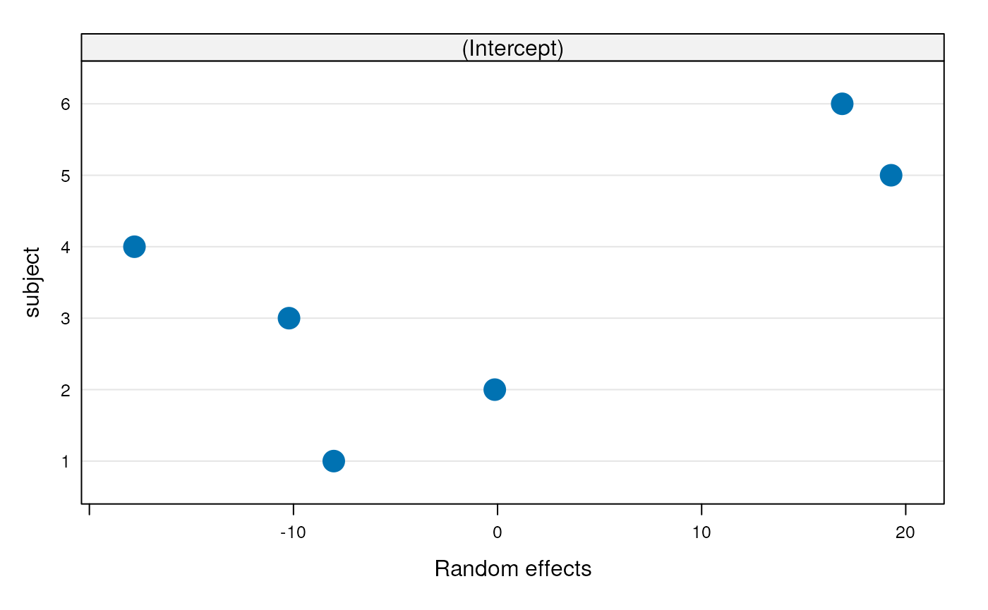
- Perform model diagnostics for random effects models
- Interpret random intercepts and random slopes
- Define and perform population average models
- Define assumptions on correlation structure in hierarchical models
- Choose between hierarchical modeling strategies
Review
Fecal fat dataset
- Lack of digestive enzymes in the intestine can cause bowel
absorption problems.
- This will be indicated by excess fat in the feces.
- Pancreatic enzyme supplements can alleviate the problem.
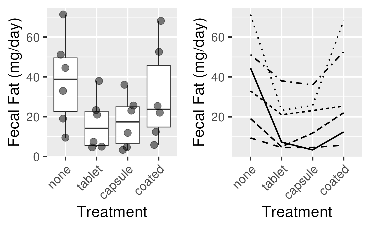
- fecfat.csv: a study of fecal fat quantity (g/day) for individuals given each of a placebo and 3 types of pills
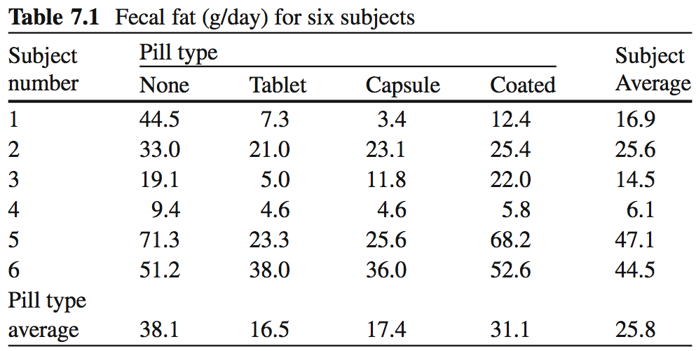
Fecal Fat dataset
Non-hierarchical analysis strategies
Non-hierarchical analysis strategies for hierarchical data
- Analyses for each subgroup
- e.g., look at each patient independently
- doesn’t work at all in this example, and in general is not an integrated analysis of the whole data
- could sort of work for an example with many patients per doctor, a few doctors
- Analysis at the highest level in the hierarchy
- first summarize data to highest level
- doesn’t work at all in this example
- could sort of work for an example with few patients per doctor, many doctors
- Analysis on “Derived Variables”
- consider each treatment type separately, take differences in fat levels between treatment/control for each patient and use paired t-tests
- can work, but not for unbalanced groups
- Fixed-effects models
When is hierarchical analysis definitely needed?
- the correlation structure is of interest, e.g. familial aggregation of disease, or consistency of treatment within centers
- we wish to “borrow strength” across the levels of a hierarchy in order to improve estimates
- dealing with unbalanced data
- we want to benefit from software designed for hierarchical data
Mixed effects models
Mixed effects models
- Model looks like two-way ANOVA:
- Assumption:
- But instead of fitting a to each individual, we assume that the subject effects are selected from a distribution of possible subject effects:
Where we assume:
- This is a mixed effects model because:
- the “true” intercept varies randomly from patient to patient
- the “true” (population) coefficient of treatment is fixed (the same for everyone)
Mixed effects model coeffients, variances, ICC
## Linear mixed-effects model fit by REML
##   Data: dat
##   Log-restricted-likelihood: -84.55594
##   Fixed: fecfat ~ pilltype
##     (Intercept)  pilltypetablet pilltypecapsule  pilltypecoated
##       38.083334      -21.550001      -20.666667       -7.016668
##
## Random effects:
##  Formula: ~1 | subject
##         (Intercept) Residual
## StdDev:    15.89557 10.34403
##
## Number of Observations: 24
## Number of Groups: 6= 0.7 = 0.7.
- Recall ICC is a measure of how large the subject effect is, in relation to the error term
- Variances were estimated directly by the model!
Assumptions of the mixed model
- Normally distributed residuals as in fixed effects model:
- Normally distributed latent variable:

Mixed effects model results
## Linear mixed-effects model fit by REML
##   Data: dat
##        AIC      BIC    logLik
##   181.1119 187.0863 -84.55594
##
## Random effects:
##  Formula: ~1 | subject
##         (Intercept) Residual
## StdDev:    15.89557 10.34403
##
## Fixed effects:  fecfat ~ pilltype
##                     Value Std.Error DF   t-value p-value
## (Intercept)      38.08333  7.742396 15  4.918805  0.0002
## pilltypetablet  -21.55000  5.972127 15 -3.608430  0.0026
## pilltypecapsule -20.66667  5.972127 15 -3.460521  0.0035
## pilltypecoated   -7.01667  5.972127 15 -1.174903  0.2583
##  Correlation:
##                 (Intr) plltypt plltypcp
## pilltypetablet  -0.386
## pilltypecapsule -0.386  0.500
## pilltypecoated  -0.386  0.500   0.500
##
## Standardized Within-Group Residuals:
##          Min           Q1          Med           Q3          Max
## -1.210052934 -0.615068039 -0.002727166  0.457105344  1.725618643
##
## Number of Observations: 24
## Number of Groups: 6- Note: correlation of the estimator of the fixed effects
- high correlations may (but not necessarily) be due to collinearity
- not usually useful, not included in output of some packages
Mixed effects model results
Inference for variance terms (and fixed effects):
## Approximate 95% confidence intervals
##
##  Fixed effects:
##                     lower       est.     upper
## (Intercept)      21.58081  38.083334 54.585860
## pilltypetablet  -34.27929 -21.550001 -8.820714
## pilltypecapsule -33.39595 -20.666667 -7.937381
## pilltypecoated  -19.74595  -7.016668  5.712618
##
##  Random Effects:
##   Level: subject
##                   lower     est.    upper
## sd((Intercept)) 8.00117 15.89557 31.57904
##
##  Within-group standard error:
##    lower     est.    upper
## 7.23240 10.34403 14.79438- Would conclude that variation of the intercept between subjects is
non-zero
- not attributable to within-subject variation
Longitudinal data
Longitudinal data
- Interested in the change in the value of a variable within a “subject”
- Collect data repeatedly through time.
- For hierarchical longitudinal analysis to be effective, before/after measurements need to be positively correlated
Longitudinal data
- Interested in the change in the value of a variable within a “subject”
- Collect data repeatedly through time.
- For hierarchical longitudinal analysis to be effective, before/after measurements need to be positively correlated
Longitudinal data examples
- Example 1: a measure of sleepiness before and after administration of treatment or placebo
- Example 2: Study of Osteoporotic Fractores (SOF dataset)
- 9,704 women tracked with clinical visits every two years
- Bone Mineral Density (BMD), Body Mass Index (BMI), many other variables
- Questions for Example 2:
- Is change in BMD related to age at menopause? This is a time-invariant predictor, age at menopause, with time-dependent changes in the outcome, BMD.
- Is change in BMD related to change in BMI? This is an analysis relating a time-varying predictor, BMI, with changes in the outcome, BMD. BMI varies quite a lot between women, but also varies within a woman over time.
Longitudinal data examples
- birthweight and birth order
- provides birthweights and order of infants from mothers who had 5
children in Georgia
- interested in whether birthweight of babies changes with order
- whether this difference depends on the mother’s age at first childbirth or on the weight of initial baby.
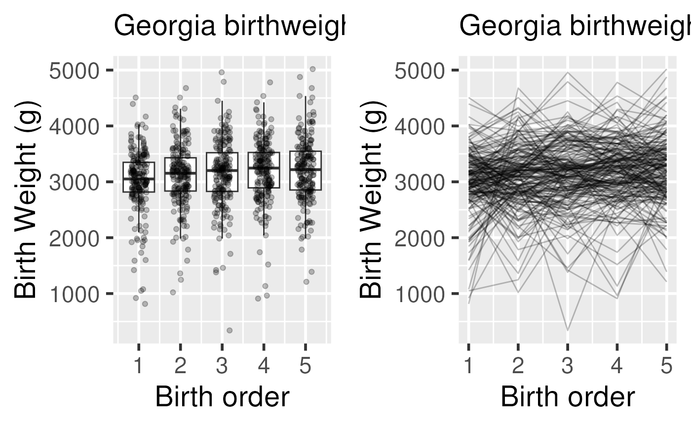
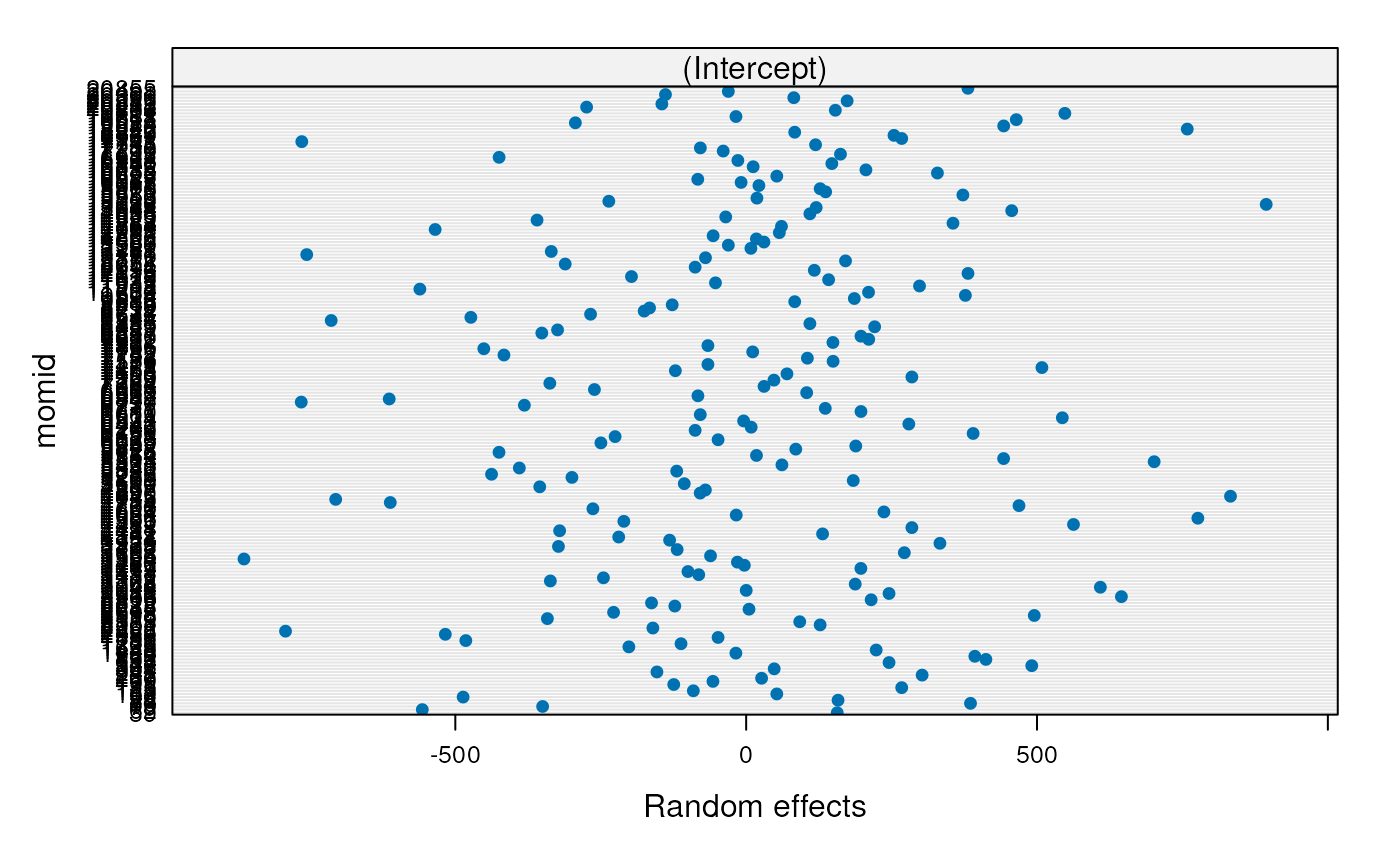
Georgia Birthweights dataset
- Does baseline birth weight vary by mother?
- random intercept
Note: there are not enough degrees of freedom to also fit a random coefficient for birth order
Georgia Birthweights dataset
summary(gafit1)## Linear mixed-effects model fit by REML
## Data: ga
## AIC BIC logLik
## 15321.65 15341.28 -7656.826
##
## Random effects:
## Formula: ~1 | momid
## (Intercept) Residual
## StdDev: 367.2676 445.0228
##
## Fixed effects: bweight ~ birthord
## Value Std.Error DF t-value p-value
## (Intercept) 2995.640 41.99615 799 71.33130 0
## birthord 46.608 9.95101 799 4.68374 0
## Correlation:
## (Intr)
## birthord -0.711
##
## Standardized Within-Group Residuals:
## Min Q1 Med Q3 Max
## -5.26801358 -0.43683345 0.05028638 0.52703429 3.30770805
##
## Number of Observations: 1000
## Number of Groups: 200Georgia Birthweights dataset
intervals(gafit1, which = "all")## Approximate 95% confidence intervals
##
## Fixed effects:
## lower est. upper
## (Intercept) 2913.20418 2995.640 3078.07582
## birthord 27.07478 46.608 66.14122
##
## Random Effects:
## Level: momid
## lower est. upper
## sd((Intercept)) 323.1724 367.2676 417.3794
##
## Within-group standard error:
## lower est. upper
## 423.7298 445.0228 467.3859- Does baseline birth weight vary by mother?
- yes: the subject variance is significantly greater than zero
- The variance between mothers is too much to be explained by within-mother variation in birth weights
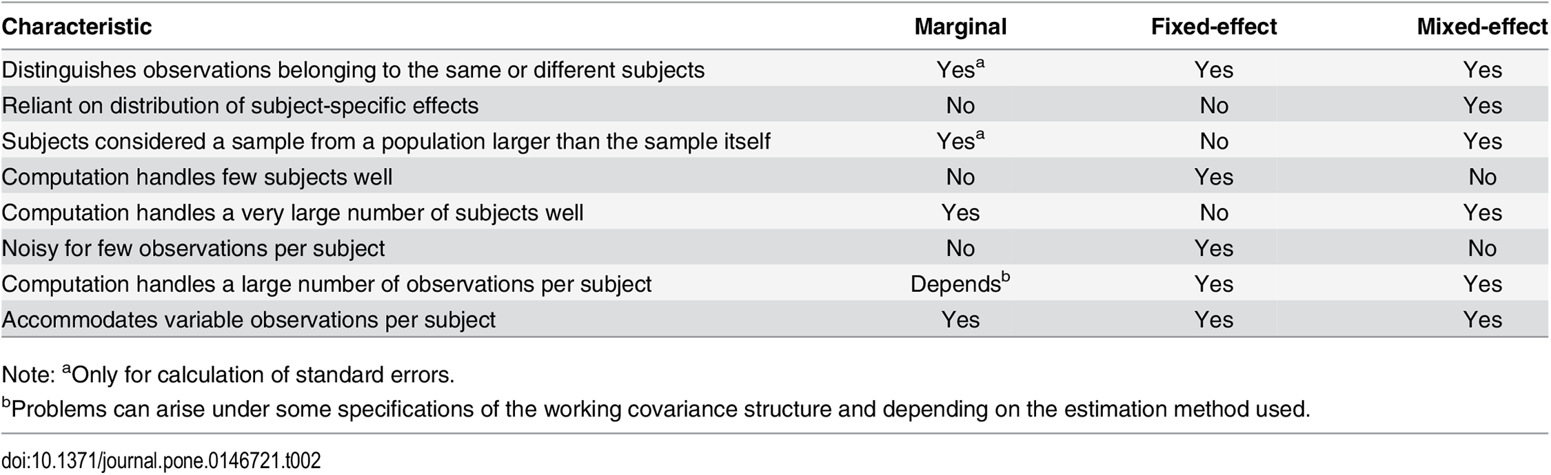
Population Average Models
Population Average Models
- An alternative to random / mixed-effects models that is more robust
to assumptions of:
- distribution of random effects
- correlation structure
- Estimates correlation structure from the data rather than assuming
normality
- Requires more clusters than observations per cluster
- Estimates regression coefficients and robust standard errors
- commonly by Generalized Estimating Equations (GEE)
Population Average Models
Compare mixed model multiple linear regression: for subject in group .
to a population average model:
Interpretations of and are equivalent
Numerically equivalent for linear and log-linear models (if specification of mixed model is correct), but not for logistic link.
Fit a population average model
gafit.gee <- gee::gee(bweight ~ birthord,
                      corstr = "exchangeable",
                      id = momid,
                      data = ga)
summary(gafit.gee)##
## GEE: GENERALIZED LINEAR MODELS FOR DEPENDENT DATA
## gee S-function, version 4.13 modified 98/01/27 (1998)
##
## Model:
## Link: Identity
## Variance to Mean Relation: Gaussian
## Correlation Structure: Exchangeable
##
## Call:
## gee::gee(formula = bweight ~ birthord, id = momid, data = ga,
## corstr = "exchangeable")
##
## Summary of Residuals:
## Min 1Q Median 3Q Max
## -2795.464 -299.126 48.840 341.144 1824.536
##
##
## Coefficients:
## Estimate Naive S.E. Naive z Robust S.E. Robust z
## (Intercept) 2995.640 41.973695 71.369462 38.808066 77.191170
## birthord 46.608 9.958128 4.680398 9.996256 4.662546
##
## Estimated Scale Parameter: 332525.3
## Number of Iterations: 1
##
## Working Correlation
## [,1] [,2] [,3] [,4] [,5]
## [1,] 1.0000000 0.4035684 0.4035684 0.4035684 0.4035684
## [2,] 0.4035684 1.0000000 0.4035684 0.4035684 0.4035684
## [3,] 0.4035684 0.4035684 1.0000000 0.4035684 0.4035684
## [4,] 0.4035684 0.4035684 0.4035684 1.0000000 0.4035684
## [5,] 0.4035684 0.4035684 0.4035684 0.4035684 1.0000000Correlation assumptions for GEE
Must make some assumption about the form of correlation among grouped observations. Some options are:
- Independence:
- no correlation between measurements within group
- Exchangeable:
- all pairwise correlations are the same (in large-N limit)
- nothing distinguishes one member of a cluster from another
- appropriate in the absence of other data structures such as measurements taken through time or space
- Auto-regressive (AR-M):
- observations taken more closely in time are more highly correlated
Correlation assumptions for GEE (cont’d)
- Unstructured:
- estimates a separate correlation between observations taken on each pair of “times”
- Non-stationary (“non_stat_M_dep”):
- similar to unstructured, but assumes all correlations for pairs separated far enough in time are zero
- Stationary (“stat_M_dep”):
- e.g. stationary of order 2: observations taken at time points 1 and 3 have the same correlation as time points 2 and 4
- but this might be different from the correlation between observations taken at times 2 and 3
- correlations for observations 3 or more time periods apart assumed to be zero
Fewer assumptions requires more data, and good assumptions improve results
Conclusions
- Ignoring within-subject correlations can produce very wrong results, and is not always “conservative”
- Hierarchical analysis strategies are needed for any of:
- When the correlation structure is of primary interest, e.g. familial aggregation of disease, or consistency of treatment within centers,
- When we wish to “borrow strength” across the levels of a hierarchy in order to improve estimates, and
- When dealing with unbalanced correlated data. E.g., no requirement that each Georgia mother have exactly 5 children.
- Population average models provide a robust alternative to mixed
models
- for one level of hierarchy
A final note on reporting results of hypothesis tests
- Include test statistic, a measure of “effect size”, and test name if unclear from test statistic
- Write in plain language and let the statistics support, not lead.
E.g.:
- do: The 36 study participants had a mean age of 27.4 (SD = 12.6), significantly older than the university mean of 21.2 years (t(35) = 2.95, p = 0.01).
- don’t: A p-value of 0.01 indicated significant difference in age of study participants compared to all university students.
- do: report confidence intervals where possible
- UW “Reporting Results of Common Statistical Tests in APA Format”: specific examples of reporting a hypothesis test result
- STROBE guidelines for reporting observational studies: https://www.strobe-statement.org/
- A Guideline for Reporting Results of Statistical Analysis in Japanese Journal of Clinical Oncology: helpful guidelines for all parts of a manuscript